- My personal website/
- Teaching Portfolio/
- Corporate strategy in a network perspective/
- Session 6 - Communities and cliques/
Session 6 - Communities and cliques

Table of Contents
Session 6 - Communities and cliques
This session marks the last ’tools’ session of the course and focuses on node communities. Communities are groupings of nodes in the network that are very densely connected with each other. Detecting communities tells us something about the overall network structure.
As always, we are working with the data set den17. We also install two packages in the beginning of our script. The purrr packages, which facilitates to work with lists, and the RcolorBrewer package, which contains a ready-to-use color palettes for creating beautiful graphics. After having loaded the packages, we can execute the usual functions to transform den17 into a graph object. See the code-snippet below:
#setting the working directory
setwd("")

# Package that makes it easier to work with lists.
install.packages("purrr")
# Package that enables you to change colors in visualizations
install.packages("RcolorBrewer")

#loading the libraries
library(tidyverse)
library(data.table)
library(ggraph)
library(igraph)
library(graphlayouts)
library(purrr)
library(RColorBrewer)

# load data
den <- read_csv("input/den17-no-nordic-letters.csv")

# subset of corporations that have a valid cvr affiliation
den1 <-
  den %>% filter(sector %in% "Corporations")

# Let us create a graph using an incidence matrix
# Create the incidence matrix
incidence <- xtabs(formula = ~ name + affiliation,
                   data = den1,
                   sparse = TRUE)

# adjacency matrix for chosing corporations
adj_c <- Matrix::t(incidence) %*% incidence

# one-mode graph for corporations
gr <- graph_from_adjacency_matrix(adj_c, mode = "undirected") %>%
  simplify(remove.multiple = TRUE, remove.loops = TRUE)

# What are the components?
complist <- components(gr)

# Decompose graph
comps <- decompose.graph(gr)

# Create an index
index <-
  table(complist$membership) %>%
  as_tibble(.name_repair = make.names) %>%
  arrange(desc(n)) %>%
  mutate(X = as.numeric(X)) %>%
  pull(1)

# Select the largest component
comp1 <- comps[[index[1]]]
6.1 Community detection
Communities are highly connected clusters of nodes within a network. The process of discovering optimal communities of nodes is called community detection. This process is an unsupervised process where each node is classified according to a community.
The most common community detection algorithm is called the Louvain clustering method, which partitions nodes by maximizing modularity.
Modularity measures how dense the connections are within subsets of vertices in a graph by comparing the density to that which would be expected from a random graph. In an unweighted and undirected graph, modularity takes a value between −0.5 and +1. Any value above zero means that the vertices inside the subgroups are more densely connected than would be expected by chance. The higher the modularity of a graph, the more connected the vertices are inside the subgroups compared to between the subgroups, and therefore the more certain we can be that the subgroups represent genuine communities of more intense connection.
Explanation are drawn from the Handbook of Graphs and Networks in People Analytics
Modularity is calculated through several steps, in which modularity is maximized. The exact process is described in this paper Blondel et al. 2008. In R, we cluster the nodes in a network by using the cluster_louvain() function.
#clustering
louvain <- cluster_louvain(comp1)

# Look inside the object
names(louvain)
## [1] "membership"  "memberships" "modularity"  "names"       "vcount"
## [6] "algorithm"
# How large are the clusters?
louvain$membership # which community does a node belong to?
##   [1]  1  2  3  4  5  1  5  6  4  6  7  8  9  4  7  6 10 11 10 10 10  2  4  6  8
##  [26] 12 13  2  6 14  2  3  5  4  7 12  3 12  4  1  8  5  1 14  2 13 13  7  3  8
##  [51]  4 13  8  3  2 10 13  4  4 10  3 14 15  4 15  1 10 15  1  4  1 10  8  3  6
##  [76]  6 13  6  3  5 10  9  4  4 10  4  2  7 10  2 13 16  2 12 12  6 14 14 10 10
## [101]  6  4 14  6  8 15  4  6  7  6  8 14  2  5  8  4 12  7  7 10 16 15  3  2  4
## [126]  4 15  3  1 10  5 15  3  3  6  6  7  3  4 10  2  2 13 12 12 10  3 13 12  8
## [151]  1 11  6  5  6  4 13 14  4  6  2 12  8  1  3  5  1  3  8  4 14  4 10  4  8
## [176] 17  8  5  7 14 10 15  1 14  4  5 15  6 17 10 13  3 10  8 12  2 15  8  4  8
## [201]  3 16  5  7  1 10 10  8 12 10  8 12  8  3  4  5  1  2  3 10 12  3  9  2  1
## [226] 10 10 10  6  2  4 12 16  8  3  4  9  4  5 14 13 12 15 16  9 10  1 13  4  5
## [251] 14  1  1  3  1  5  2  2 15 15  9 13  3  3  3  3  1 14  2  6  9 13  4 10  6
## [276]  1  2 12 12  5  3  7  4  6  7  4  8  8 15  8 14 15  3  5 17  3  2 17  2  1
## [301]  6 12 10 16  4  2 11 15  6 13  3  4  7  7  1 10 15  1 15  4  5 13 12 10 13
## [326] 10  7 10  6 10 13 13 13  7  5  4  7 14  1 16 15 15  1  1 12 10 10  1  4  4
## [351]  3  3  8  7  1  1  3 15  3 10 10 10 10 10  7  1  1  1  7 16  4  5 14 13 14
## [376]  3  8  5  9  3  4  1  2  2  3  4 13 17 17  3  2  3 13  1 12  3  4  2 15 12
## [401] 16  6 13  2 14  1 12  7 16 14 13  3 15 10  9 10 16  9 13 13  1  5  8  1  1
## [426] 10 10  8  9 11  4  7  8 14  4  3  3 14  6  3 12 12 10 10 12  2 14  3 15  4
## [451]  3 14  2  6  4 15 15 12 10  3  3  3  3  3  7  3 14 16 13  6  5  4  7 14  3
## [476]  5  1  7 13  3 10 10 12 10  1 12  2 14 10  7  6  4  4  4 12  3 10 14  1  3
## [501]  4  1 10 10 10 10 13  2 10 10  2 10 10 10  5  7 13  6  3 10 12  2  1 10  3
## [526] 13  8  1  1  8  4  1 15
unique(louvain$membership) %>% length() # number of communities
## [1] 17
table(louvain$membership) # distribution of members
##
##  1  2  3  4  5  6  7  8  9 10 11 12 13 14 15 16 17
## 47 36 59 55 26 32 28 31 11 66  4 32 33 28 27 12  6
# How many clustering iterations?
dim(louvain$memberships)
## [1] 3 533
# How effective has it clustered?
louvain$modularity # 3 rounds of clustering
## [1] 0.5753514 0.6820413 0.6933936
modularity(louvain) # last round
## [1] 0.6933936
As we can see, the algorithm has found 17 distinct communities (which may deviate at your personal computer) in three clustering rounds. In each clustering iteration, the modularity has been increased, and has reached the value 0.69 in the last round.
6.2 Community visualization
As always, we are interested not only in community calculation, but also in how to visualize them. This is simply done by adding the community scores to a network object. In this case, we create a new network attribute called V(comp1)$community.
To make it visually more pleasing, we run a loop with the map2_chr() function which creates an edge attribute E(comp1)$community. This edge attribute gives the edge the same community color if it connects two nodes within an community, and gives it a black color if it connects two different communities.
# Do they have the same sequence of names?
all.equal(louvain$names, V(comp1)$name)
## [1] TRUE
# adding membership as an attribute to community (with sprintf() function which makes membership values look nicer)
V(comp1)$community <- sprintf("%02d",louvain$membership)

# DOES NOT NEED TO BE UNDERSTOOD --
# Creating edge attribute that gives the edge the same community color if it connects two nodes within an community, and gives it a black color if it connects two different communities.

a1 <- as_tibble(as_edgelist(comp1), .repair_names = "unique")

E(comp1)$community <-
  # mapping two edge cols in a function into a character vector (chr)
  map2_chr(a1$V1, a1$V2, function(.x, .y){
    # if else statement
  ifelse(
    # checks if community between nodes that form edges (in a1 object) are part of the same communtiy
    V(comp1)$community[which(V(comp1)$name==.x)] ==
      V(comp1)$community[which(V(comp1)$name==.y)],
    # if yes, write the community
    V(comp1)$community[which(V(comp1)$name==.x)],
    # if not, write "9999"
    "9999")
})
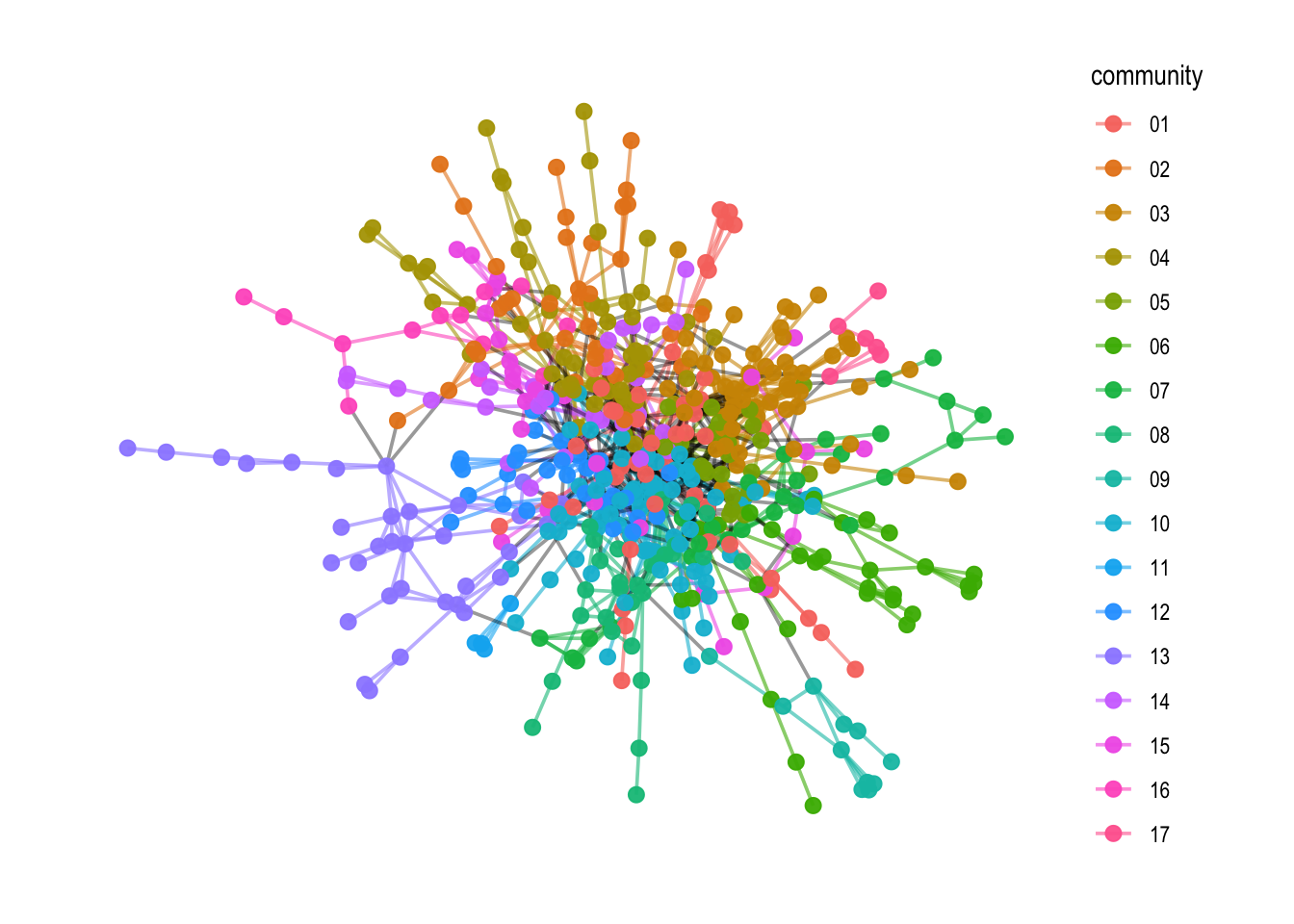
Now, this can be visualized with the ggraph() plotting syntax.
# Plotting
comp1 %>%
  ggraph(layout = "fr") +
  geom_edge_link0(aes(filter=community!= "9999",
                      color = community),
                  width = 0.65,
                  alpha = 0.6) +
  geom_edge_link0(aes(filter=community == "9999"),
                  color = "black",
                  width = 0.65,
                  alpha = 0.4) +
  geom_node_point(aes(color=community),
                  alpha=0.95,
                  size=2.5) +
  theme_graph()
## Warning: Using the `size` aesthetic in this geom was deprecated in ggplot2 3.4.0.
## ℹ Please use `linewidth` in the `default_aes` field and elsewhere instead.
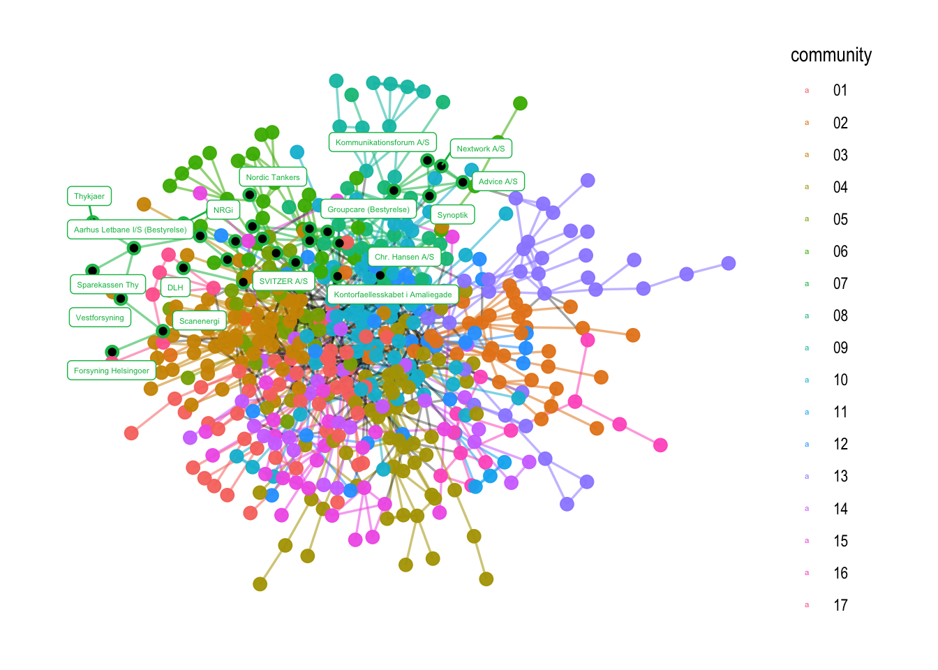
6.2.1 Understanding community membership
Sometimes, it might be difficult to see who is a part of each community. The best way of finding the nodes that are part of the community is to make a tibble with two columns, name and community. You can however, also pull the names directly for each community and then label their names in a graph. This is what I am doing in the code below:
# to find the nodes who are a part of a given community. Here, I am looking at hte members of community nr. 07
names_c7 <- V(comp1)$name[which(V(comp1)$community == "07")]

# to visualize them in the graph
comp1 %>%
  ggraph(layout = "stress") +
  geom_edge_link0(aes(filter=community!='9999', color=community), width=0.6, alpha=0.55) +
  geom_edge_link0(aes(filter=community=='9999'), color='black', width=0.6, alpha=0.35) +
  geom_node_point(aes(color=community), alpha=0.95, size=3) +
  geom_node_point(aes(filter=name %in% names_c7), color = "black", size=1.5) +
  geom_node_label(aes(filter=name %in% names_c7, label=name, color=community), size = 1.5, repel=TRUE, force = 10) +
  theme_graph()
6.2.2 Changing colors
Sometimes, the default color palettes are not visually pleasing. You have two options to change color palettes:
- if there are not many unique colors present, I recommend using the viridis functions
scale_color_viridis()orscale_edge_color_viridis()as a part of yourggraph()workflow - if many colors are present, use the RColorBrewer palettes
You can display all of the given color palettes by calling the function display.brewer.all(). Make sure that you have installed the package and called library(RcolorBrewer) before using this function.
display.brewer.all()
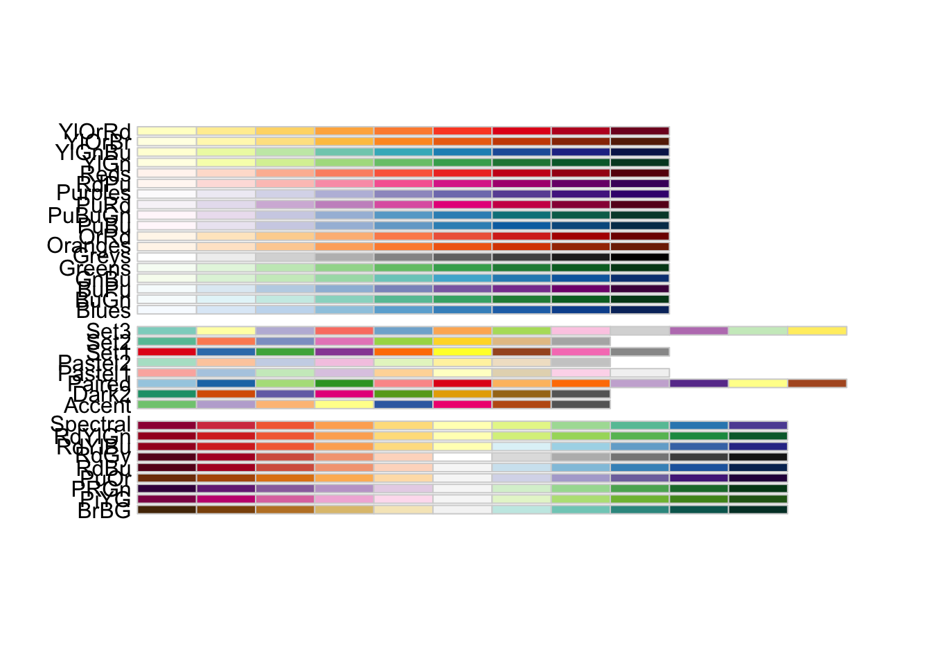
If you have chosen a palette that you like, you can also adapt the amount of different colors you need with the following functions. This can then be used in the ggraph() syntax.
# choose color and adapt to the amount of different colors you need
amount <- V(comp1)$community %>% unique() %>% length()
mycolors <- colorRampPalette(brewer.pal(8, "Paired"))(amount)

comp1 %>%
  ggraph("fr") +
  geom_edge_link0(aes(filter=community!='9999',
                      color=community),
                  width=0.6,
                  alpha=0.55) +
  geom_edge_link0(aes(filter=community=='9999'),
                  color='black',
                  width=0.6,
                  alpha=0.35) +
  geom_node_point(aes(color=community),
                  alpha=0.95,
                  size=3) +
  scale_edge_color_manual(values = mycolors) +
  # use this function to change the color palette
  scale_color_manual(values = mycolors) +
  theme_graph()

6.3 Cliques
Cliques are subsets of nodes in a graph whose edge density equals 1 meaning that every member is connected with each other. This makes cliques the most extreme kind of community in an undirected graph. In comparison to community detection, clique membership can be overlapping.
We find cliques with the cliques() function where we need to specify the lower size threshold. The minimum value must be 2 as we need at least two nodes to form a clique.
# How to find cliques:
clique <- cliques(comp1, min = 2) # specify min 2 as there should be at least two people (exclude isolates)

# How many do we have?
length(clique)
## [1] 2797
# How many of them have a different size?
map_dbl(.x = clique, ~ length(.x)) %>% table()
## .
##    2    3    4    5    6    7    8
## 1244  867  445  176   53   11    1
For strategic inquiries, such as how to find all cliques that Sydbank is included in, we can use the keep() function of the purrr package that allows us to find names in lists.
# For strategic queries:
# Example: to find how many cliques Sydbank is in.
a1 <- keep(.x = clique, ~ any(.x$name == "Sydbank"))


# How large are the cliques that Sydbank is in?
map_dbl(.x = a1, ~length(.x)) %>% table()
## .
##  2  3  4  5  6  7
## 13 22 22 15  6  1
Last, we can also use the maximal.cliques() function to find the maximal non-overlapping amount of cliques in a network.
# how many max. cliques are there?
count_max_cliques(comp1, min = 2)
## [1] 499
# find all of the maximal cliques
max_cliques <- maximal.cliques(comp1, min = 2)

# look at the distribution

# distribution?
map_dbl(.x = max_cliques, ~ length(.x)) %>% table()
## .
##   2   3   4   5   6   7   8
## 262 138  58  33   4   3   1