- My personal website/
- Teaching Portfolio/
- Corporate strategy in a network perspective/
- Session 5 - Brokerage and assortativity/
Session 5 - Brokerage and assortativity

Table of Contents
Session 5 - Brokerage and assortativity
This session connects to session 4 which introduced analysis tools for the node level. Here, we further investigate the broker role with Burt’s constraint as a measure for brokerage. Second, we cover assortativity which measures homophily among nodes - or in other words, the likelihood that nodes with similar properties are connected with each other.
But first, after having set working directory and loaded packages, we load our data set, create a graph object and select the biggest component.
# load data
den <- read_csv("input/den17-no-nordic-letters.csv")

# subset of corporations that have a valid cvr affiliation
den1 <-
  den %>% filter(sector %in% "Corporations")

# Let us create a graph using an incidence matrix
# Create the incidence matrix
incidence <- xtabs(formula = ~ name + affiliation,
                   data = den1,
                   sparse = TRUE)

# adjacency matrix for chosing corporations
adj_c <- Matrix::t(incidence) %*% incidence

# one-mode graph for corporations
gr <- graph_from_adjacency_matrix(adj_c, mode = "undirected") %>%
  simplify(remove.multiple = TRUE, remove.loops = TRUE)

# What are the components?
complist <- components(gr)

# Decompose graph
comps <- decompose.graph(gr)

# Create an index
index <-
  table(complist$membership) %>%
  as_tibble(.name_repair = make.names) %>%
  arrange(desc(n)) %>%
  mutate(X = as.numeric(X)) %>%
  pull(1)

# Select the largest component
comp1 <- comps[[index[1]]]
5.1 Burt’s constraint
Burt’s constraint is a measure of brokerage. The idea of brokerage suggests that nodes who occupy structural holes in a network have greater access to resources and can exert more influence over other nodes who they are connected to. Higher values of Burt’s constraint signify that nodes have less structural opportunities for bridging structural holes in the network. It measures how many direct ties of a node are redundant - the more nodes are redundant, the more constraint a node is.
# constraint - the higher, the less chances for brokerage
constraint(comp1)[1:10]
##                            3C Groups                                  3xN
##                            1.0000000                            0.8650000
##                  5E Byg (Bestyrelse)                                   7N
##                            0.5000000                            0.6087572
##                            A-pressen                A.P. Moeller - Maersk
##                            0.2290325                            0.1502256
##        A/S DANSK ERHVERVSINVESTERING                    Aalborg Forsyning
##                            1.0000000                            0.5000000
##                Aalborg Stiftstidende Aalborg Zoologiske Have (Bestyrelse)
##                            1.0000000                            0.5000000
# make brokerage variable so we can compare it to the other measures
brokerage <- 1- constraint(comp1)

# Let us make a data.frame with tibble() and look at the different measures.
metrics <- tibble(

  name = names(constraint(comp1)),
  brokerage = 1- constraint(comp1),
  betweenness = betweenness(comp1, directed = FALSE),
  degree = degree(comp1, mode = "all")

)

# Let us see who is least constraint?
metrics %>% arrange(desc(brokerage))
## # A tibble: 533 × 4
##    name                                           brokerage betweenness degree
##    <chr>                                              <dbl>       <dbl>  <dbl>
##  1 Tryg                                               0.911      11793.     20
##  2 Industriens Pension                                0.905       6273.     19
##  3 DLR Kredit                                         0.904       8371.     23
##  4 MAJ INVEST HOLDING A/S                             0.894       6080.     18
##  5 Nykredit Holding A/S (bestyrelse)                  0.884       6480.     18
##  6 Schouw & Co.                                       0.883      11209.     17
##  7 Big Future (Advisroy Board)                        0.881       4795.     12
##  8 Arbejdernes Landsbank                              0.880       4092.     17
##  9 TOTALKREDIT A/S                                    0.880       3778.     20
## 10 Koebenhavns Lufthavns Vaekstkomité (Medlemmer)     0.880       3831.     12
## # … with 523 more rows
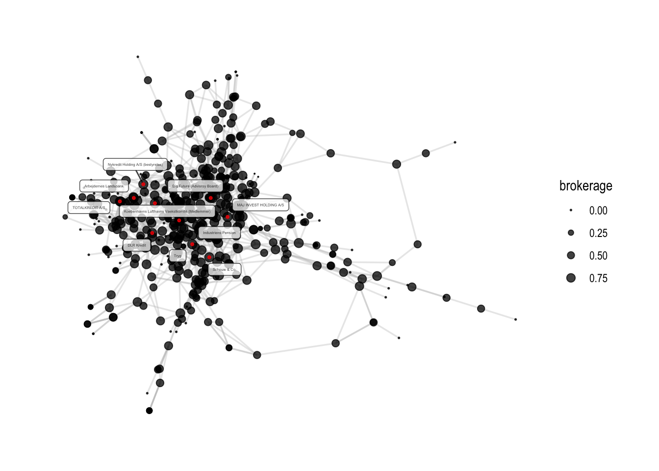
As you can see, Burt’s constraint is very similar to betweenness, with certain distinctions. In a sense, Burt’s constraint is more local, not taking the whole network structure into account.
Let us visualize Burt’s constraint by adding it as a graph attribute.
# Make sure to test if sequence is correct before adding it to a network attribute.
all.equal(metrics$name, V(comp1)$name)
## [1] TRUE
# Add to our graph object
V(comp1)$brokerage <- metrics$brokerage

# how to select the 10 most central people?
ten_largest <- metrics %>%
  arrange(desc(brokerage)) %>% #arranage by brokerage
  slice(1:10) %>% # slice the data frame and look at the first 10 nodes
  pull(name) # extract only the names

# visualize
comp1 %>%
  ggraph(layout = "mds") +
  geom_edge_link0(color='grey', width=0.6, alpha=0.35) +
  geom_node_point(aes(size=brokerage), alpha=0.75) +
  # scalling the size interval of geom node point
  scale_size(range = c(0.01,3)) +
  scale_color_viridis() +
  geom_node_label(aes(filter=name %in% ten_largest, label=name), alpha=0.75, repel=T, size=1) +
  geom_node_point(aes(filter=name %in% ten_largest), color='red', size=.75, alpha=0.75) +
  theme_graph()
## Warning: Using the `size` aesthetic in this geom was deprecated in ggplot2 3.4.0.
## ℹ Please use `linewidth` in the `default_aes` field and elsewhere instead.
5.2 Assortativity
Assortativity measures the extend to which nodes with similar properties are connected to each other. The assortativity coefficient ranges between -1 and 1, where 1 indicates that there is a high likelihood of two nodes with the same properties being connected. Networks that have an assortativity of 0 are usually referred to as neutral.
There are three kinds of assortativities we cover in this session:
categorical assortativity which measures to what extend nodes with the same categorical properties are connected with each other. This is measured by the function
assortativity_nominal()continuous assortativity which is used to measure homophily based on a continuous variable with the function
assortativity()assortativity degree with calculates the if nodes with similar degree scores are connected with each other. This is measured with the function
assortativity_degree()
5.2.1 Continuous assortativity
In order to show examples of calculating the former options, I will create a new variable which measures the gender proportion in an company board. This will create the basis for the calculation of assortativity().
# What is the gender proportion?
den1 %>% count(gender)
## # A tibble: 4 × 2
##   gender        n
##   <chr>     <int>
## 1 Binominal    30
## 2 Men        6605
## 3 Women      1305
## 4 <NA>         49
# Let's aggregate gender proportions for each affiliation (but only look at women and men)
gender <- den1 %>%
  #filter for women and men only
  filter(gender %in% c("Women", "Men")) %>%
  #count amount of women and men per affiliation
  count(affiliation, gender) %>%
  # do something, but group by affiliation first
  group_by(affiliation) %>%
  # generates the total number of board members per affiliation
  mutate(n_total = sum(n),
         # generates the share of women and men.
         share = n/(sum(n)))

# Now, let us focus on one share: the share of men in the dataset.
Men <- gender %>% filter(gender == "Men")
Women <- gender %>% filter(gender == "Women" & n == n_total)
Women$share = 0

Men <- Men %>% select(affiliation, share)
Women <- Women %>% select(affiliation, share)

# create a common object
gender1 <- rbind(Men, Women)

# now, just choose those affiliations that are part of the biggest component
gender2 <-
  gender1 %>%
  filter(affiliation %in% V(comp1)$name)


# check if they are same than the comp1aph
all.equal(gender2$affiliation, V(comp1)$name)
## [1] "457 string mismatches"
index <- match(V(comp1)$name, gender2$affiliation)
gender2 <- gender2 %>% arrange(factor(affiliation, levels = affiliation[index]))
all.equal(gender2$affiliation, names(V(comp1)))
## [1] TRUE
# Let us add gender share as an attribute to the graph
V(comp1)$share_men <- gender2$share

# Visualize
comp1 %>%
  ggraph(layout = "stress") +
  geom_edge_link0(width=.5, alpha=0.4) +
  geom_node_point(aes(color=share_men), size=5) +
  theme_graph() +
  # make a gradient of color from red to blue per gender
  scale_color_gradient2(low='firebrick4', mid='grey80', high='dodgerblue4', midpoint=0.5, na.value='pink')
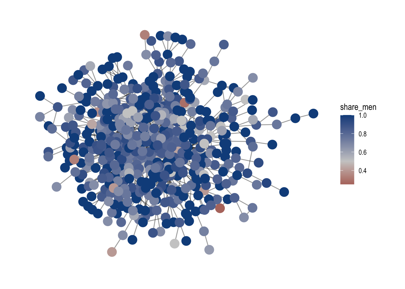
# Calculate assortativity for share of men
assortativity(comp1, V(comp1)$share_men, directed=FALSE)
## [1] 0.1578647
In this example, the assortativity of 0.157tells us that there is a small likelihood that boards with a similar gender proportion are directly connected with each other.
5.2.2 Categorical assortativity
Now, we can use the gender proportion variable to create a new categorical variable of gender. It changes the variable to female dominated, gender_balanced and male_dominated depending on their proportions. This is then used to calculate and visualize categorical assortativity.
# let us create a categorical gender variable based on gender2.
gender3 <-
  gender2 %>%
  # we are creating a new variable "gender_cat" where we use a case_when() statement
  mutate(gender_cat = case_when(
    # when the share col has a share of males below 0.45, it is female dominated
    share < 0.45 ~ "female_dominated",
    0.45 < share & share < 0.55 ~ "gender_balanced",
    .default = "male_dominated"))

# let us add it to the graph comp1
all.equal(gender3$affiliation, names(V(comp1)))
## [1] TRUE
V(comp1)$gender_cat <- gender3$gender_cat

comp1 %>%
  ggraph(layout = "fr") +
  geom_edge_link0(width=.5, alpha=0.4) +
  geom_node_point(aes(color=gender_cat), size=3) +
  scale_color_manual(values = c("salmon1", "olivedrab", "steelblue")) +
  theme_graph()
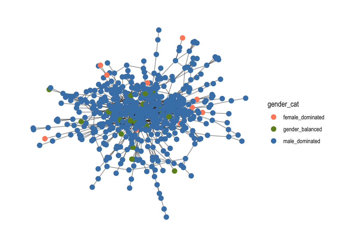
# Make sure to write as.factor(), so it is recognized as a categorical variable
assortativity_nominal(comp1,
                      as.numeric(as.factor(V(comp1)$gender_cat)),
                      directed = FALSE)
## [1] 0.0395072
With an assortativity of 0.039, there is a neutral likelihood that nodes with the same gender category gender_cat are directly connected with each other. The score is telling us that we cannot expect boards with the same gender proportion to be connected with each other.