- My personal website/
- Teaching Portfolio/
- Corporate strategy in a network perspective/
- Session 2: Network components, density and paths/
Session 2: Network components, density and paths

Table of Contents
2.1 Loading packages and data
We start where we ended session 02. Since we create a new r-script, we also need to load the packages and the data again. We install a new package called graphlayouts.
# load working directory
setwd("/Users/alexandergamerdinger/Library/CloudStorage/OneDrive-CBS-CopenhagenBusinessSchool/PhD/teaching/virksomhedsstrategi_2023")

# install new packages

install.packages('graphlayouts')

# loading libraries
library(data.table)
library(tidyverse)
library(igraph)
library(ggraph)
library(graphlayouts)

# load den17 from the input folder.

den <- read_csv("input/den17-no-nordic-letters.csv")

# we'll be looking only at corporations

den1 <- den %>% filter(sector == "Corporations")
2.1.1 Making data subset
Similar to session 01, we are interested in looking at the corporations subset only, which we specify with the filter() function. However, this time, we want to further subset the data tibble to only include those individuals in the data set that appear at least twice.
To do this, we make use of the group_by() function which allows us to group our data set into “homogeneous” blocks before perform any operation on them. Here, we group by name.
Next, we use the mutate() function to add a new variable to the data set. In the mutate function, we specify the name of the new column before the equality sign, and then specify the operations with which the old column is mutated by after the sign. Here, we simply want to count the number of rows by group with the n() function.
Last, we filter the N column to select only those individuals, who appear in the data set more than once. We assign the series of modifications of den1 to the the object den2.
# select only the people who are in the data at least twice
# create a new variable, with tidyverse.

den2 <- den1 %>%
  # group by the column "name"
  group_by(name) %>%
  # create a new variable called "N" and fill it with the number of rows per group
  mutate(N = n()) %>%
  # this is a function to reorder columns, and to place the N function as first col of the data set
  select(N, everything()) %>%
  # now, filter by the new column variable and select those, who are in the data set more than once.
  filter(N > 1)
2.1.2 Creating corporations graph object
After having modified out data set, we now create a graph object. For this, we re-use code from session 01.
# Create incidence matrix
# Sparse T means that instead of 0, it will just make a "."
incidence <- xtabs(formula = ~ name + affiliation, data = den2, sparse = TRUE)

adj_c <- Matrix::t(incidence) %*% incidence

# load a corporation network object and call it "gr". Then, simplify it, to get rid of self-loops and weights

gr <- graph_from_adjacency_matrix(adj_c, mode = "undirected") %>%
  simplify(remove.multiple = TRUE, remove.loops = TRUE)

#view graph object
gr
## IGRAPH 69d5696 UN-- 661 1332 --
## + attr: name (v/c)
## + edges from 69d5696 (vertex names):
## [1] 3C Groups          --Nielsen & Nielsen Holding
## [2] 3xN                --Hildebrandt & Brandi
## [3] 3xN                --Lead Agency
## [4] 5E Byg (Bestyrelse)--E 3-Gruppen
## [5] 5E Byg (Bestyrelse)--T. Hansen Gruppen
## [6] 7N                 --Brdr. A. & O. Johansen (AO)
## [7] 7N                 --Kontorfaellesskabet paa Sankt Annae Plads
## [8] A-pressen          --Arbejdernes Landsbank
## + ... omitted several edges
2.2 Density
The density of a network is a measure that tells us about the probability that two random nodes of the network are linked with each other. It is calculated by dividing the given number of edges by the total possible number of edges. A complete graph, for example, would have a density of 1.
Here are some examples:
Full Graph
e1 <- make_full_graph(40)
plot(e1, vertex.size=10, vertex.label=NA)
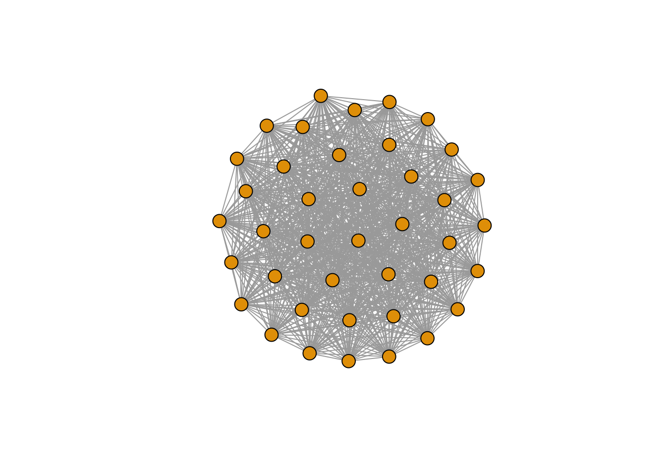
edge_density(e1, loops=FALSE)
## [1] 1
Star Graph
e2 <- make_star(40)
plot(e2, vertex.size=10, vertex.label=NA)
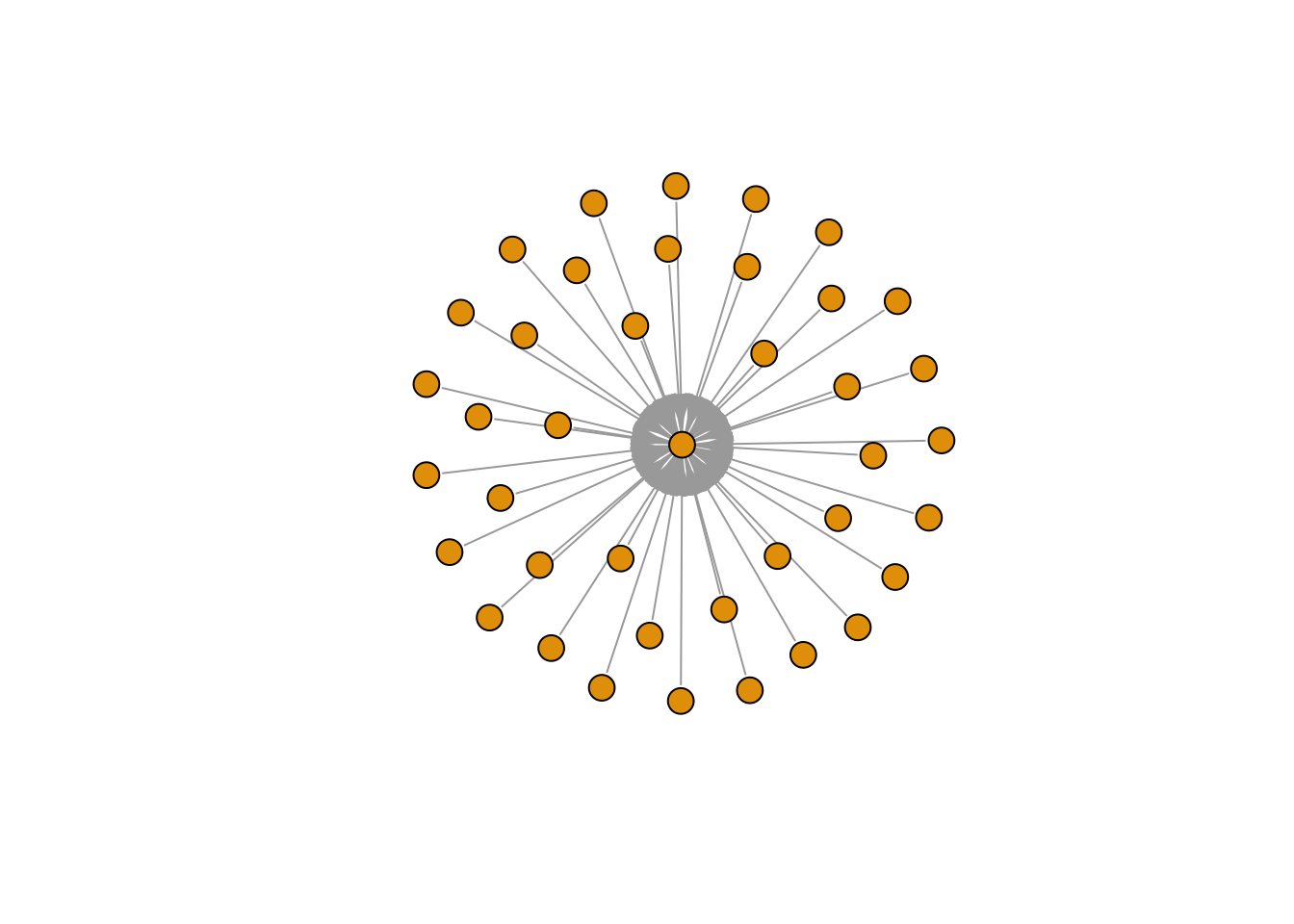
edge_density(e2, loops=FALSE)
## [1] 0.025
Tree Graph
e3 <- make_tree(40, children = 3, mode = "undirected") # try putting 'out' or 'in' in the mode-argument
plot(e3, vertex.size=10, vertex.label=NA)
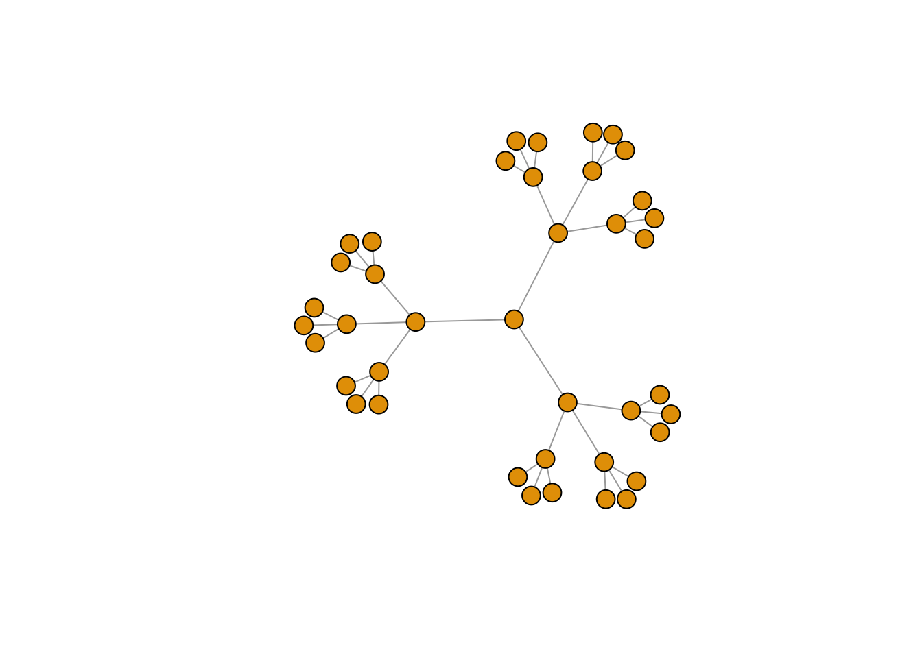
edge_density(e3, loops=FALSE)
## [1] 0.05
If we calculate the density of our graph object gr then we find it at 0.01. For those of you, who wonder why we add the argument loop = FALSE in the edge_density() function; this is because we only deal with simplified networks without self-loops. Hence, we need to add this argument.
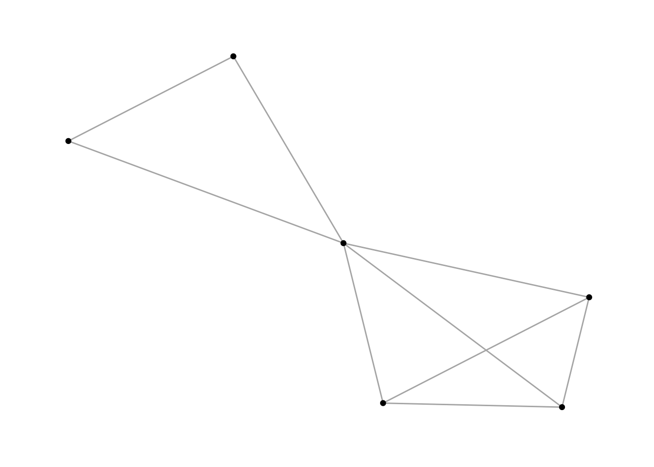
2.3 Components of a graph
The component of a graph is also called a connected sub-graph. Here is an example of graph components:

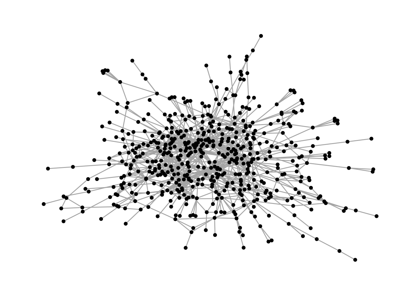
The graph object gr, which has 661 nodes and1332 ties, looks like this if we visualize it:
# plot
gr %>%
  ggraph(layout = "fr") +
  geom_edge_link0(color = "gray70") +
  geom_node_point(size=1.5) +
  theme_graph()
## Warning: Using the `size` aesthetic in this geom was deprecated in ggplot2 3.4.0.
## ℹ Please use `linewidth` in the `default_aes` field and elsewhere instead.
## This warning is displayed once every 8 hours.
## Call `lifecycle::last_lifecycle_warnings()` to see where this warning was
## generated.
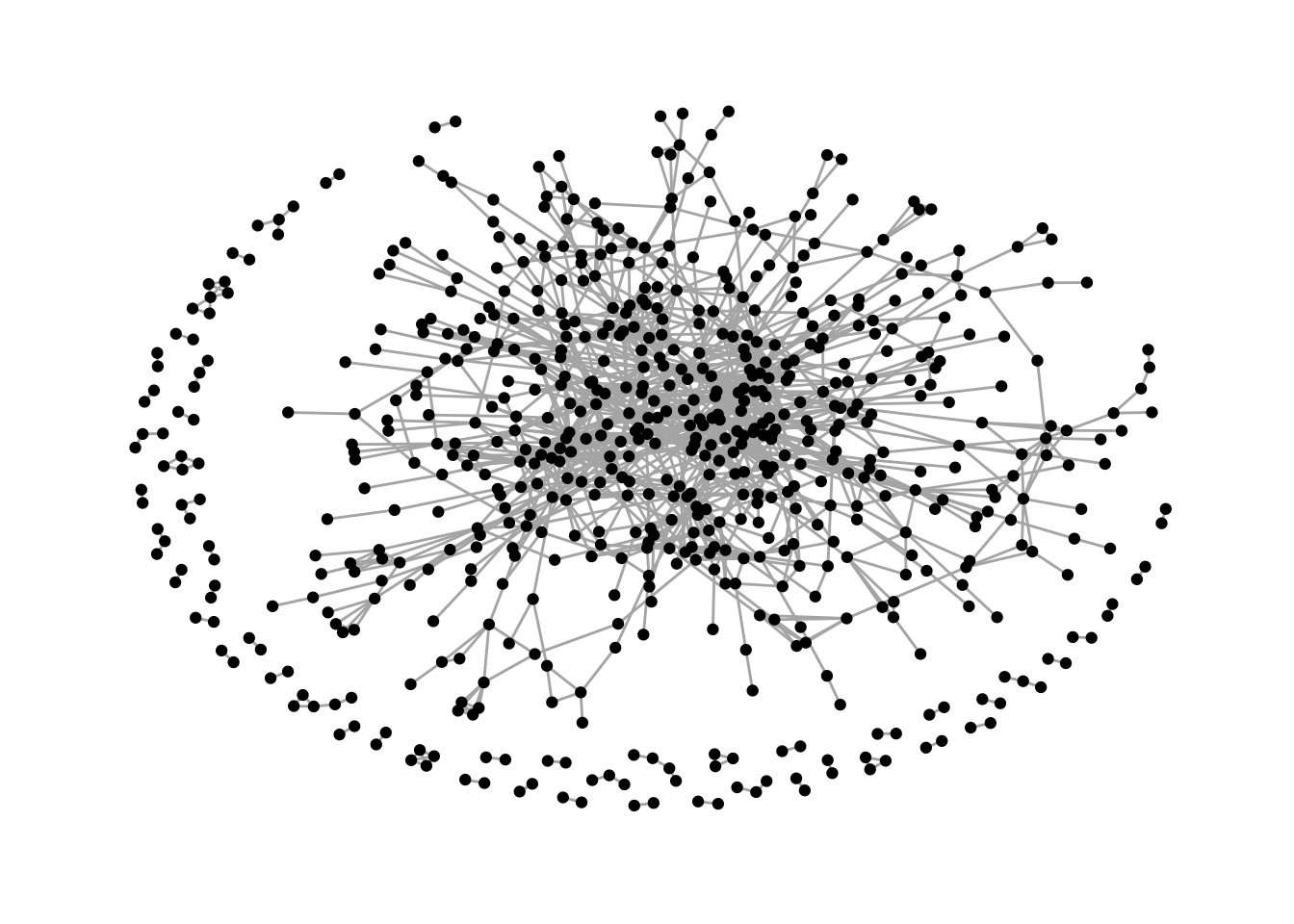
As we can see, there is a main graph component in the middle of the visualization, a few small components on the edges of the graph object.
In this case, it is interesting to look at the biggest component of the graph. We can get an overview over all components of a graph with the igraph function components().
This function generates a list containing the following vectors:
membership, which is a vector assigning each node to a numbered componentcsize, which returns the size of each componentno, which is the number of connected components
# what are the components
complist <- components(gr)

# what does they contain?
complist$membership[1:20] # notice that I am only looking at the first 20 because it is a massive vector
##                            3C Groups                                  3xN
##                                    1                                    1
##                  5E Byg (Bestyrelse)                                   7N
##                                    1                                    1
##                            A-pressen                  A. Enggaard Holding
##                                    1                                    2
##                A.P. Moeller - Maersk        A/S DANSK ERHVERVSINVESTERING
##                                    1                                    1
##     Aalborg Engineering (bestyrelse)                    Aalborg Forsyning
##                                    3                                    1
##                Aalborg Stiftstidende Aalborg Zoologiske Have (Bestyrelse)
##                                    1                                    1
##      Aarhus Letbane I/S (Bestyrelse)                             Aarsleff
##                                    1                                    1
##         Accura Advokatpartnerselskab                       Actona Company
##                                    4                                    1
##    Adserballe & Knudsen (Bestyrelse)                 Advance (Bestyrelse)
##                                    5                                    1
##                           Advice A/S                      AGRO SUPPLY A/S
##                                    1                                    1
complist$csize
##  [1] 533   2   4   3   4   2   3   2   2   3   3   4   6   4   2   2   2   2   2
## [20]   2   5   2   2   2   2   2   3   2   2   2   2   2   2   3   3   2   3   2
## [39]   2   2   2   2   2   2   3   2   2   2   2   2   2   2   2
complist$no
## [1] 53
To actually decompose the graph, and visualize the biggest and next biggest component, we use the function decompose.graph() which renders a list of small graph components.
Since we are interested in choosing the biggest component, we need to make sure that we select the correct graph component. This is done using a little trick, namely by tabulating complist$membership and then sorting it, and creating an index which is further used to select the biggest graph component.
# the decomposed graph - you are welcome to take a look if you want - but be wanted, it is a long list.
comps <- decompose.graph(gr)
## Warning: `decompose.graph()` was deprecated in igraph 2.0.0.
## ℹ Please use `decompose()` instead.
## This warning is displayed once every 8 hours.
## Call `lifecycle::last_lifecycle_warnings()` to see where this warning was
## generated.
# create an index
index <-
  # tabulate complist$membership
  table(complist$membership) %>%
  # save as tibble
  as_tibble(.name_repair = make.names) %>%
  # make X numeric
  mutate(X = as.numeric(X)) %>%
  # sort
  arrange(desc(n)) %>%
  # pull the vector
  pull(1)
The object index shows the position of the graph components in comps ordered from biggest graph component to smallest. So, index[1] reflects the position in comps which contains the biggest component, index[2] reflects the position in comps with the second biggest component, and so on…
To get the actual graph object, we just need to select it in comps and then assign it to a new name.
#largest component
comp1 <- comps[[index[1]]]

#second largest component
comp2 <- comps[[index[2]]]
After finding the components, we can now calculate their edge density by writing edge_density(comp1, loops = FALSE). We can also visualize them:
comp1 %>%
  ggraph(layout = "fr") +
  geom_edge_link0(color = "gray70") +
  geom_node_point(size=1.5) +
  theme_graph()
comp2 %>%
  ggraph(layout = "fr") +
  geom_edge_link0(color = "gray70") +
  geom_node_point(size=1.5) +
  theme_graph()
2.3.1 How to find people and affiliations in components?
A natural question that arises when cutting the graph into components is: How do I find out more about the members?
This is done in the following way:
# in names, we store all affiliation names from the second largest component
names <- V(comp2)$name

# who are the people (and all of their attributes) that are a part of these boards?
den2 %>%
  filter(affiliation %in% names) %>%
  view()

# or look at everyone in the same affiliations from original data set.
den %>%
  filter(affiliation %in% names) %>%
  view()
2.4 Transitivity
Transitivity is a measure that represents the number of actual triads out of all possible triads in the network. Thereby, it measures the existence of tightly connected communities. To understand the measure a little better, take a look at these graphs:
# a ring graph, which does not contain any triads
g1 <- make_ring(10)
plot(g1)
transitivity(g1) # 0 - no triads
## [1] 0
# a sample graph
g2 <- sample_gnp(10, 4/10)
plot(g2)
transitivity(g2)
## [1] 0.2571429
Let us calculate the transitivity of the whole graph gr and the biggest component comp1.
transitivity(gr)
## [1] 0.3115276
transitivity(comp1)
## [1] 0.3089441
2.5 Path Lengths
The path length between two nodes is simply the sum of the weights of the edges traversed in the path. If a graph does not have any weights, it is assumed to be equal to 1. Since we are here looking at an unweighted graph, the length of the path is the number of edges traversed on that path.
Path lengths between nodes
To get the path lengths between all nodes in the network, we simply use the distances() function. To view a matrix with all distances, type distances(comp1) %>% view()
Mean distances
To get the mean distances between nodes in a component, try the following:
# mean distance of the biggest comp1
mean_distance(comp1)
## [1] 5.168073
# iterates through mean distances of all of the components
map_dbl(comps, mean_distance)
##  [1] 5.168073 1.000000 1.666667 1.333333 1.000000 1.000000 1.333333 1.000000
##  [9] 1.000000 1.333333 1.333333 1.500000 1.400000 1.166667 1.000000 1.000000
## [17] 1.000000 1.000000 1.000000 1.000000 1.700000 1.000000 1.000000 1.000000
## [25] 1.000000 1.000000 1.000000 1.000000 1.000000 1.000000 1.000000 1.000000
## [33] 1.000000 1.000000 1.333333 1.000000 1.333333 1.000000 1.000000 1.000000
## [41] 1.000000 1.000000 1.000000 1.000000 1.333333 1.000000 1.000000 1.000000
## [49] 1.000000 1.000000 1.000000 1.000000 1.000000
Distances between two specific nodes
To calculate the distance from specific node to all other nodes in a graph component, we use the following function:
distances <-
  # distances function
  distances(comp1,
            # origin
            v = which(V(comp1)$name =="LEGO A/S"),
            # to
            to = V(comp1))

# to view the object

# view(distances)
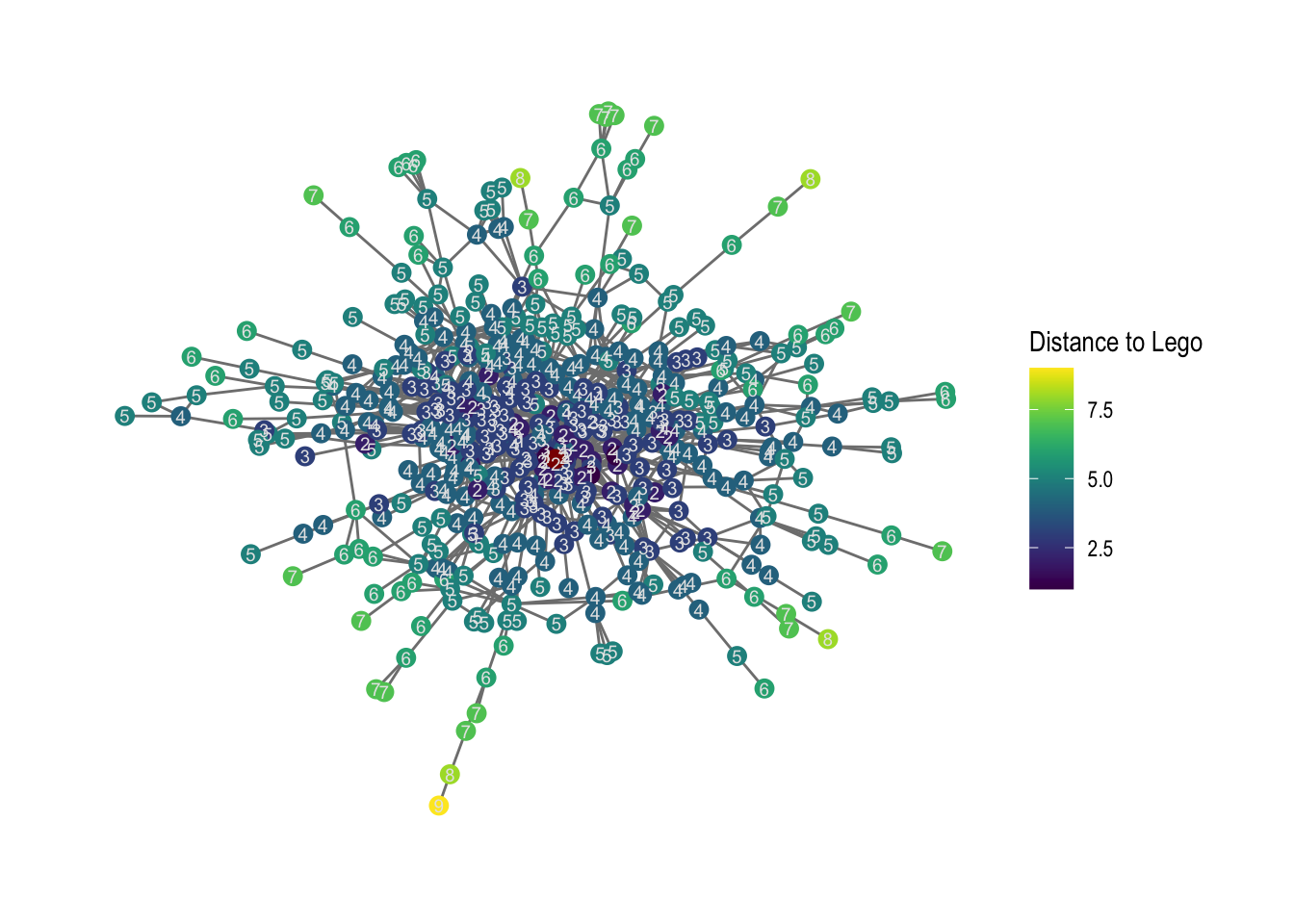
Having retrieved these distances is informative, but maybe a little hard to imagine. Let us spend some time in visualizing this in a network graph. For this, we create two network attributes:
the network attribute
distancewhich shows the distance betweenLEGO A/Sand every other node in the grapha logical network attribute
legowhich specifies where in the networkLEGO A/Scan be found
This is how we operate it in R.
# first, we check if the cols of the distances object are equal to the names of the graph object

all.equal(target = colnames(distances),
          current = names(V(comp1)))
## [1] TRUE
# let us add a new graph attribute. It is a vertex (node) attribute, and hence, it has to include V(comp1).
# So first, we create $distance and assign distances to it

V(comp1)$distance <- as.numeric(distances)

# and now, we create a second attribute, which is called lego, which is TRUE only if LEGO A/S appears

V(comp1)$lego <- ifelse(
  # the condition
  names(V(comp1)) == "LEGO A/S",
  # what happens if condition is true
  TRUE,
  # what happens if it is not
  FALSE)
Let us plot this.
library(tidygraph)
##
## Attaching package: 'tidygraph'
## The following object is masked from 'package:igraph':
##
##     groups
## The following object is masked from 'package:stats':
##
##     filter
comp1 %>%
  ggraph(layout = "fr") +
  geom_edge_link0(color="gray50") +
  # filtering for FALSE, which is not LEGO
  geom_node_point(aes(filter=lego==FALSE,
                      color=distance), size =3) +
  # filtering for TRUE, which is LEGO
  geom_node_point(aes(filter=lego==TRUE),
                  color="darkred", size=3) +
  # distances as text for all nodes that are not lego
  geom_node_text(aes(filter=lego==FALSE,
                     label = distance),
                 color= "gray90", size=2.5) +
  # to change the legend
  labs(color = "Distance to Lego") +
  # to scale colors
  scale_color_viridis() +
  theme_graph()
# save it - we save it in our output folder.
ggsave("output/02-distance_to_lego.png", width = 30, height = 17.5, units = "cm")
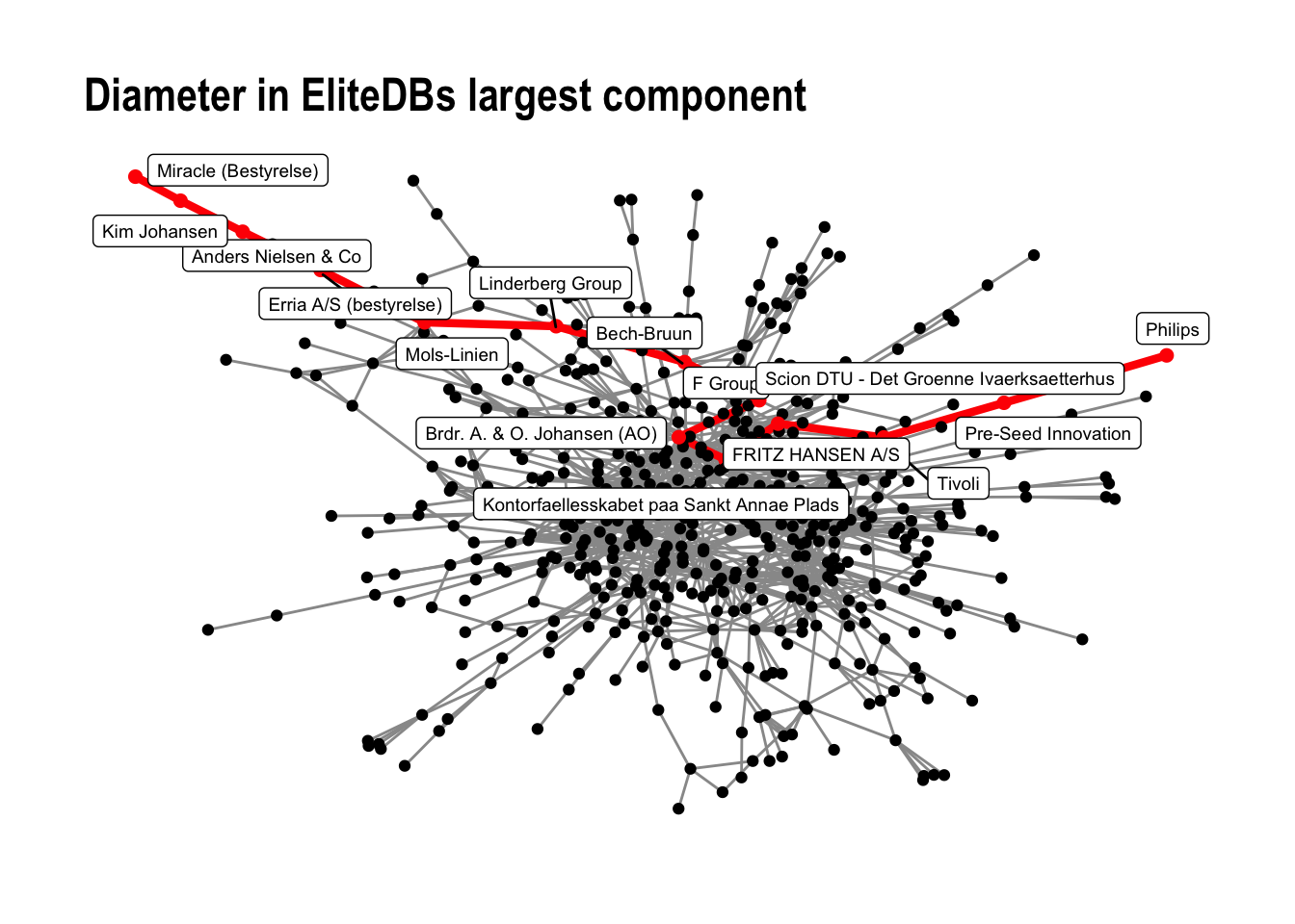
2.6 Diameter
The diameter is a measure that only makes sense to use in connected graph components. It is the shortest path in the network. Networks with smaller diameters are often considered close communities. The shortest path in the network is calculated using the following functions:
# diameter for the network component
diameter(comp1, directed = FALSE)
## [1] 14
# Who is on the outskirts?
farthest.nodes(comp1, directed = FALSE)
## Warning: `farthest.nodes()` was deprecated in igraph 2.0.0.
## ℹ Please use `farthest_vertices()` instead.
## This warning is displayed once every 8 hours.
## Call `lifecycle::last_lifecycle_warnings()` to see where this warning was
## generated.
## $vertices
## + 2/533 vertices, named, from f0ce197:
## [1] Miracle (Bestyrelse) Philips
##
## $distance
## [1] 14
# How to traverse it?
diam <- get.diameter(comp1, directed = FALSE)
## Warning: `get.diameter()` was deprecated in igraph 2.0.0.
## ℹ Please use `get_diameter()` instead.
## This warning is displayed once every 8 hours.
## Call `lifecycle::last_lifecycle_warnings()` to see where this warning was
## generated.
diam
## + 15/533 vertices, named, from f0ce197:
##  [1] Miracle (Bestyrelse)
##  [2] Kim Johansen
##  [3] Anders Nielsen & Co
##  [4] Erria A/S (bestyrelse)
##  [5] Mols-Linien
##  [6] Linderberg Group
##  [7] Bech-Bruun
##  [8] F Group
##  [9] Brdr. A. & O. Johansen (AO)
## [10] Kontorfaellesskabet paa Sankt Annae Plads
## + ... omitted several vertices
Now, if we want to visualize the diameter, we need to first create two network attributes. A vertex attribute V(comp1)$diameter as well as an edge attribute E(comp1)$diameter
# making new graph attribute for nodes
V(comp1)$diameter <-
    # condition to evaluate
  ifelse(V(comp1)$name %in% names(diam),
         # if condition is true
         TRUE,
         # if condition is false
         FALSE)

# making new graph attribute for edges. The code for edges are kind of different, this is igraph-specific
E(comp1)$diameter <- FALSE
E(comp1, path = diam)$diameter <- TRUE
Now, we can visualize this:
# plot it
comp1 %>%
  ggraph(layout = "fr") +
  geom_edge_link0(aes(filter=diameter==FALSE), color = "gray60") +
  geom_edge_link0(aes(filter=diameter==TRUE), color = "red", width = 1.5) +
  geom_node_point(aes(filter=diameter==FALSE), color = "black") +
  geom_node_point(aes(filter=diameter==TRUE), color = "red", size =2) +
  geom_node_label(aes(filter=diameter==TRUE, label = name), nudge_y = -0.3, size =2.5, repel = TRUE) +
  labs(title = 'Diameter in EliteDBs largest component') +
  theme_graph()
And then, save the figure in the output folder.
# save the output to the output folder
ggsave("output/02-diameter_comp1.png", width = 30, height = 17.5, units = "cm")
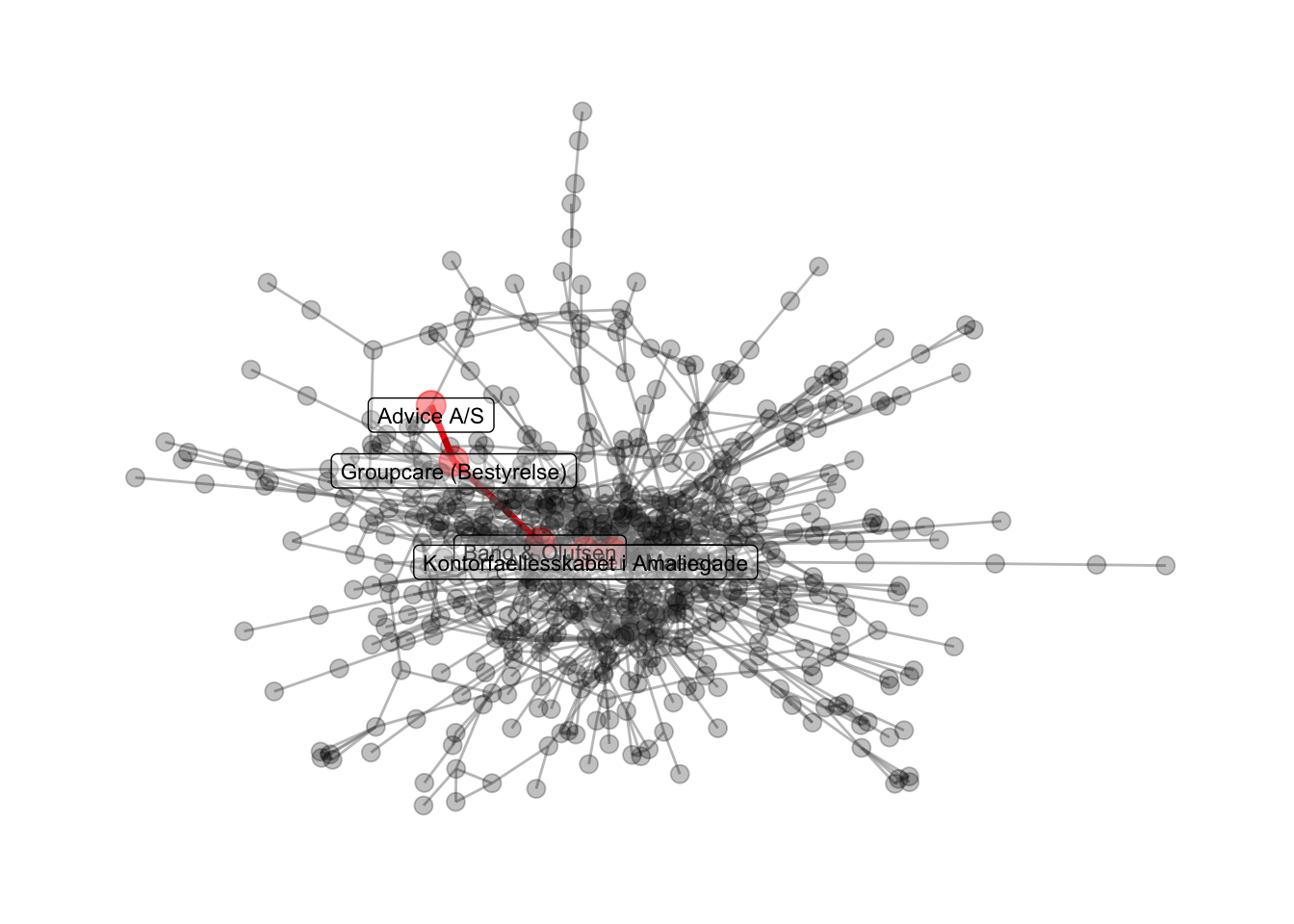
2.7 Highlighting certain paths
Last, we can highlight the shortest path between two specific nodes in a connected network. First, we make the path and add this path as a network attribute.
# get the igraph object that contains the path
path_of_interest <- shortest_paths(comp1,
                            from = names(V(comp1)) =="A.P. Moeller - Maersk",
                             to  = names(V(comp1)) =="Advice A/S",
                             output = "both") # both path nodes and edges

# path_of_interest object gives us a path for nodes ($vpath) and one for edges ($epath)
path_of_interest
## $vpath
## $vpath[[1]]
## + 5/533 vertices, named, from f0ce197:
## [1] A.P. Moeller - Maersk            Kontorfaellesskabet i Amaliegade
## [3] Bang & Olufsen                   Groupcare (Bestyrelse)
## [5] Advice A/S
##
##
## $epath
## $epath[[1]]
## + 4/1244 edges from f0ce197 (vertex names):
## [1] A.P. Moeller - Maersk--Kontorfaellesskabet i Amaliegade
## [2] Bang & Olufsen       --Kontorfaellesskabet i Amaliegade
## [3] Bang & Olufsen       --Groupcare (Bestyrelse)
## [4] Advice A/S           --Groupcare (Bestyrelse)
##
##
## $predecessors
## NULL
##
## $inbound_edges
## NULL
# making new graph attribute for nodes
V(comp1)$path1 <-
    # condition to evaluate
  ifelse(V(comp1)$name %in% names(path_of_interest$vpath[[1]]),
         # if condition is true
         TRUE,
         # if condition is false
         FALSE)

# making new graph attribute for edges.
E(comp1)$path1 <- FALSE
E(comp1, path = path_of_interest$vpath[[1]])$path1 <- TRUE
Second, we visualize this, and save it in our output folder.
comp1 %>%
ggraph(layout='fr') +
geom_edge_link0(aes(filter=path1==TRUE), color='red', width=1.2) +
geom_edge_link0(aes(filter=path1==FALSE), color='grey50', alpha=0.5) +
geom_node_point(aes(filter=path1==TRUE), color='red', size=5, alpha=0.5) +
geom_node_point(aes(filter=path1==FALSE), color='black', size=3, alpha=0.25) +
geom_node_label(aes(filter=path1==TRUE, label=name), color='black', size=3, alpha=0.25, nudge_y=-1) +
theme_graph()
# save to the output folder
ggsave('output/lektion02-path-example.png', width=30, height=17.5, unit='cm')