Session 4 - Analysis of node centrality measures

Table of Contents

Session 4 - Analysis of node centrality measures #

This session will provide you with tools to analyze important nodes in a network. It is different from session 2, which focused on the analysis of the network structure, as we are now focusing on the node level importance.

Before we introduce the new measures, let us set our working directory, load den17, find a subset and load a network object.

## load working directory 
setwd("")

# libs
library(data.table)
library(tidyverse)
library(igraph)
library(ggraph)
library(readxl)
library(writexl)
library(graphlayouts)
source("r/custom_functions.R")

# Load and manipulate data set --------------------------------------------
# Load
den <- read_csv("input/den17-no-nordic-letters.csv")

# we'll be looking only at corporations
den1 <- 
  den %>% 
  filter(sector == "Corporations") 

# Now, let us only select linkers
den2 <- 
  den1 %>% 
  group_by(name) %>% 
  mutate(N = n()) %>% 
  select(N, everything()) %>% 
  filter(N >1 ) 

# Let us create a graph using an incidence matrix
# Create the incidence matrix
incidence <- xtabs(formula = ~ name + affiliation, 
                   data = den2, 
                   sparse = TRUE)

# adjacency matrix
adj_c <- Matrix::t(incidence) %*% incidence

# one-mode graph 
gr <- graph_from_adjacency_matrix(adj_c, mode = "undirected") %>% 
  simplify(remove.multiple = TRUE, remove.loops = TRUE)

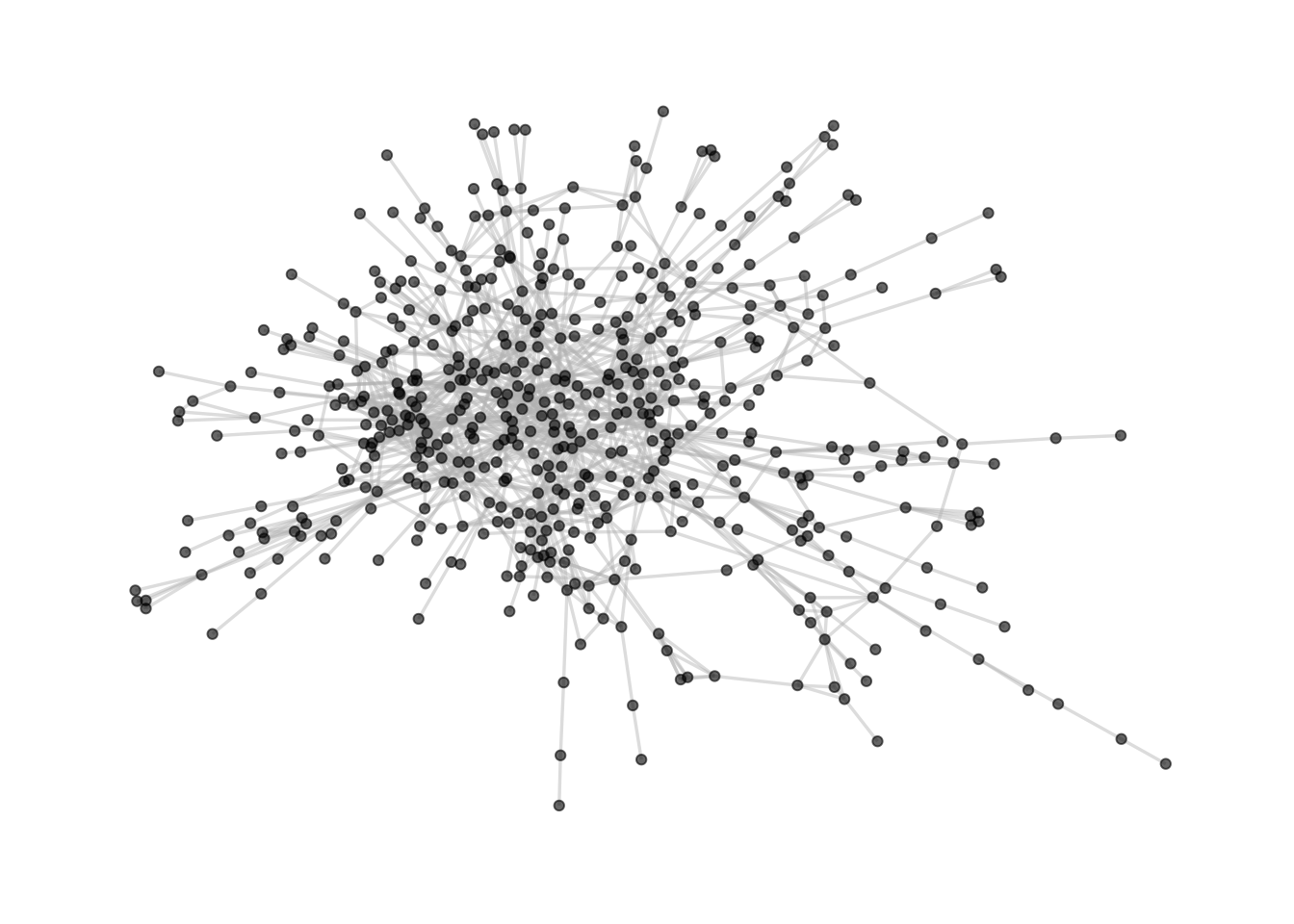
After we have loaded our graph object gr we also want to find the largest component comp1. We use the following code to do that.

# What are the components?
complist <- components(gr)

# Decompose graph
comps <- decompose.graph(gr)

# Create an index
index <- 
  table(complist$membership) %>% 
  as_tibble(.name_repair = make.names) %>% 
  arrange(desc(n)) %>% 
  mutate(X = as.numeric(X)) %>% 
  pull(1)

# Select the largest component
comp1 <- comps[[index[1]]] 

# plot 
comp1 %>% 
ggraph(layout='fr') + 
geom_edge_link0(color='grey', width=0.6, alpha=0.45) + 
geom_node_point(color='black', alpha=0.6)  + 
theme_graph()

4.1 Centrality measures #

In this session will focus on the following centrality measures:

Degree centrality, which measures the amount of direct links that a node has with others. It tells us something about the local centrality of a node and is calculated with the function degree()
Betweenness centrality, which measures how important a given node is in connecting other pairs of nodes in the graph. It is a common measure for identifying brokers in a network and is calculated with the function betweenness()
Closeness centrality, which measures how efficiently the entire graph can be traversed from a given node. Nodes with high closeness centrality are likely to reach the entire network more efficiently. It is calculated with the function closeness()
Eigenvector centrality which measures how connected a node is to other influential nodes. Nodes can have high influence through being connected to a lot of other nodes with low influence, or through being connected to a small number of highly influential nodes. It is calculated with the function eigen_centrality()

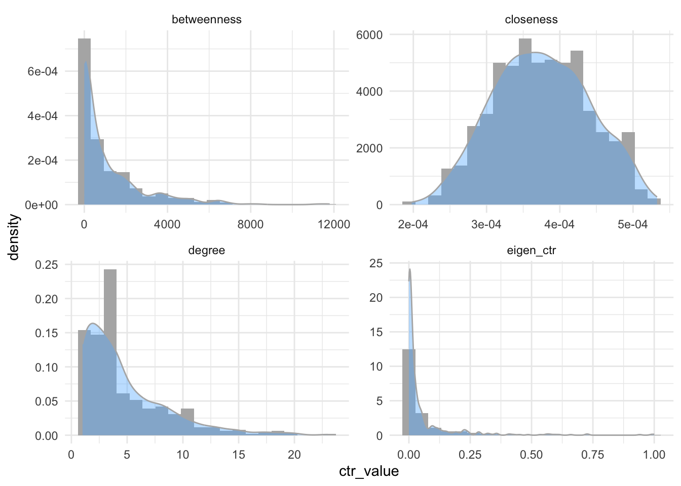
Let us compare the measures with each other. First, we create a table called metrics which contains all centrality metrics.

Second, we look at the distributions of these metrics. You are not obliged to understand this ggplot() code. More importantly, you see that while betweenness, degree and eigenvector centrality behave similarly, closeness is almost normally distributed.

# create a table with all centrality metrics
metrics <- tibble(
  name = names(degree(comp1, mode="all")),
  degree =        degree(comp1, mode="all"),
  betweenness =   betweenness(comp1, directed=FALSE),
  closeness =     closeness(comp1, mode="all"), 
  eigen_ctr =         eigen_centrality(comp1, directed=FALSE)$vector
)

# look at the tibble 
head(metrics)

## # A tibble: 6 × 5
##   name                  degree betweenness closeness eigen_ctr
##   <chr>                  <dbl>       <dbl>     <dbl>     <dbl>
## 1 3C Groups                  1          0   0.000332   0.00226
## 2 3xN                        2          0   0.000354   0.00273
## 3 5E Byg (Bestyrelse)        2        531   0.000323   0.00509
## 4 7N                         2          0   0.000416   0.0174 
## 5 A-pressen                  9        422.  0.000446   0.285  
## 6 A.P. Moeller - Maersk     11       3547.  0.000464   0.0923

# look at the distributions
metrics %>% 
  # changing tibble format 
  pivot_longer(degree:eigen_ctr, 
               values_to = "ctr_value", 
               names_to = "ctr_names") %>% 
  # ggplot
  ggplot(aes(x = ctr_value, y = after_stat(density), group = ctr_names, )) +
  geom_histogram(bins = 20, fill = "gray70") +
  geom_density(alpha=0.4, fill = "steelblue1", color = "gray70") +
  # spreads it out to four panes 
  facet_wrap(~ctr_names, scales = "free" ) +
  theme_minimal()

Next, we will add some additional columns to further understand the relationship between the centrality scores. We will make a column where we include the size of the affiliation, and create a ranking system telling us the overall rank of a node by each centrality measure. Again, this code is a little advanced and not meant to be reproduced by you, so just focus on the interpretation.

# Count the number of individuals per affiliation and filter by those that are in the metrics tibble
a1 <- den %>% 
  # count the affiliations
  count(affiliation, sort = TRUE) %>% 
  # filter
  filter(affiliation %in% metrics$name) %>% 
  # rename to metge
  rename(N = n, name = affiliation)

# merge with net_metrics data set 
metrics <- 
metrics %>% 
  left_join(a1, by = "name") %>% #merge by left data.frame which is net_metrics
  select(name, N, everything())

# make measure index
m1 <- c('degree', 'betweenness', 'closeness', 'eigen_ctr')

for (i in m1) {
  metrics <- metrics %>% arrange(desc(get(i)))
  metrics <- metrics %>% mutate(!!paste0(i, "_rank") := rleid(get(i)))
}

# Making a new variable called sum_rank, and arranging the dataset by this new variable
metrics <- 
metrics %>% 
  mutate(sum_rank = degree_rank+betweenness_rank+closeness_rank+eigen_ctr_rank) %>% 
  arrange(sum_rank)

# take a look at metrics 
head(metrics)

## # A tibble: 6 × 11
##   name          N degree betwe…¹ close…² eigen…³ degre…⁴ betwe…⁵ close…⁶ eigen…⁷
##   <chr>     <int>  <dbl>   <dbl>   <dbl>   <dbl>   <int>   <int>   <int>   <int>
## 1 DLR Kred…    13     23   8371. 5.18e-4   0.989       1       3       3       2
## 2 Tryg         14     20  11793. 5.33e-4   0.405       2       1       1      17
## 3 Nykredit…    17     18   6480. 4.99e-4   0.595       4       9       9       8
## 4 Industri…    15     19   6273. 5.09e-4   0.412       3      13       7      16
## 5 MAJ INVE…     8     18   6080. 5.21e-4   0.316       4      14       2      24
## 6 Kirkbi (…     6     15   4818. 5.13e-4   0.358       7      25       5      19
## # … with 1 more variable: sum_rank <int>, and abbreviated variable names
## #   ¹betweenness, ²closeness, ³eigen_ctr, ⁴degree_rank, ⁵betweenness_rank,
## #   ⁶closeness_rank, ⁷eigen_ctr_rank

After running this snipped, look at the metircs object with the view() function to further understand the association between the centrality metrics.

4.2 Network visualization #

After having looked at the different centrality measures, the next step is to include them into network visualizations. Before we add a new graph attributes, it is always important to check if the sequence of items is the same between the graph object and the attribute vector.

In case the sequence is not the same, we use the match() functions to change the order of a vector and the factor() function to change the order of a data frame.

# be sure that the names of the affiliations are the same and sorted the same way
all.equal(metrics$name, V(comp1)$name) # woups

## [1] "533 string mismatches"

# however, they are just in a different order
all.equal(sort(metrics$name),sort(V(comp1)$name))

## [1] TRUE

# We need to match these two values 
# The match function reproduces the order (in numerical location) of the first vector, to the second one. 
index <- match(V(comp1)$name,metrics$name)

new_order <- metrics$name[index] #see for yourself

all.equal(new_order, V(comp1)$name) # now it is the same order.

## [1] TRUE

# we can also reorder the whole data frame
metrics <- metrics %>% arrange(factor(name, levels = name[index]))

all.equal(metrics$name, V(comp1)$name)

## [1] TRUE

After we have found the correct sequence, we can add the centrality measures as a node attribute to our graph object comp1.

# add the attributes / variables
V(comp1)$size <- metrics$N
V(comp1)$closeness <- metrics$closeness
V(comp1)$betweenness <- metrics$betweenness

Last, we can visualize the centrality measures as part of the graph object. In the first example, nodes are colored by betweenness scores, while in the second example, they are colored by closeness. Last, both graph objects are saved.

# Visualizing by betweenness 
comp1 %>% 
  ggraph(layout='fr') + 
  geom_edge_link0(color='grey', width=0.6, alpha=0.35) + 
  geom_node_point(aes(color=betweenness, size=size), alpha=0.75) +
  scale_color_viridis() +
  geom_node_label(aes(
  filter=name %in% {metrics %>% filter(betweenness_rank < 10) %>% pull(name)} #baseR version would be: net_metrics$name[net_metrics$betweenness_rank < 10]
,label=name), alpha=0.65, size = 3, repel=T, force = 50) +
  theme_graph()

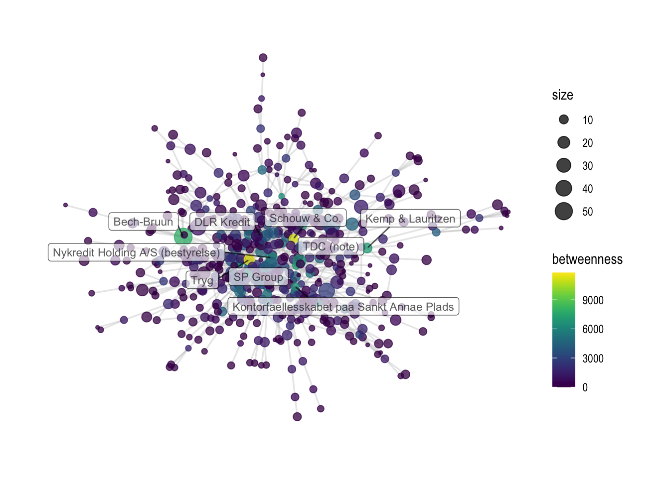
ggsave('output/elitedb-graph-betweenness.png', width=30, height=17.5, unit='cm')

# another example, with closeness
comp1 %>% 
  ggraph(layout='fr') + 
  geom_edge_link0(color='grey', width=0.6, alpha=0.35) + 
  geom_node_point(aes(color=closeness, size=size), alpha=0.75) + 
  theme_graph() + scale_color_viridis() +
  geom_node_label(aes(
    filter=name %in% {metrics %>% filter(grepl("bank", tolower(name))) %>% pull(name)},
    label=name), alpha=0.65, repel=T,size=3, force = 50)

## Warning: ggrepel: 12 unlabeled data points (too many overlaps). Consider
## increasing max.overlaps

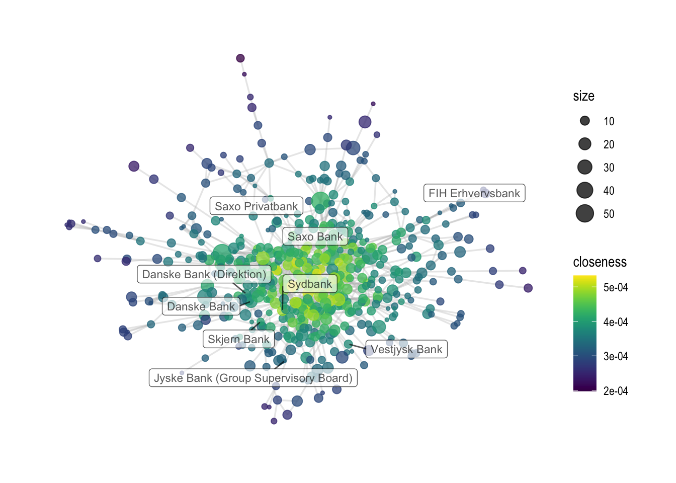
ggsave('output/elitedb-graph-closeness.png', width=30, height=17.5, unit='cm')