Session 1: Introduction to network analysis

Table of Contents

Session 1 - Introduction to network analysis #

The first thing you need to do is to set a project folder called virksomhedsstrategi which you can either place on your desktop, or into a another folder (such as one called 6_semester).

In this folder, I would like you to create 4 new sub-folders. Make sure that all of these are spelled with small caps, to make typing easier.

a folder called input where you will all the data files (in csv, xlsx, or other formats)
a folder called outputwhere you will save all network figures we will produce
a folder called rwhere you will save all your r-scripts. Make sure to make an r-script for each of the sessions.

After you have created all of the folders, you can open your Rstudio. Create a new r-script, and set your working directory to the file virksomhedsstrategi.

For macOs users, click on the folder name, and press Option + CMD + C. Paste the path into the function setwd(). It should look something similar to this:

setwd("/Users/alexandergamerdinger/Library/CloudStorage/OneDrive-CBS-CopenhagenBusinessSchool/PhD/teaching/virksomhedsstrategi_2023")

1.1 Installing and loading packages #

After you have set your working directory, we will install and load important packages that we will use throughout the course.

The tidyverse package, which is basically a collection of a variety of packages that makes it easy and visually pleasing to manipulate and work with data
The igraphpackage, which allows us to construct network objects
The ggraphpackage, which enables us to create beautiful network graphs
The data.table package, which we will use occasionally for some data wrangling

How do we install and load packages? Please note that packages need to only be installed once. This means that you can simply delete the install.packages() function right after its execution.

# install packages (but only run this once)
install.packages("tidyverse")
install.packages("igraph")
install.packages("ggraph")
install.packages("data.table")

# load pckages (run this every time you open/re-open your r-script)
library("tidyverse")
library("igraph")
library("ggraph")
library("data.table")

1.1.1 A note on the tidyverse syntax #

The tidyverse package is great because it has transformed the way of writing R, and has made it much more beautiful. One very important aspect of the package is the use of the pipe %>%.

The pipe allows us to write cleaner and more visually pleasing code. Let us take a look at this data set iris with the attempt to find the mean petal length and width of all species above a petal width of 0.2.

In baseR you would have to write this:

#finding a sub set
subset <- subset(iris, Petal.Width > 0.2)

# selecting only columns on Petals
only_pedal <- subset[,c("Petal.Length", "Petal.Width", "Species")]

# finding mean Petal length and width per species
aggregate(subset[ ,c("Petal.Length", "Petal.Width")],
          by = list(subset$Species), 
          FUN = mean)

##      Group.1 Petal.Length Petal.Width
## 1     setosa      1.51875       0.375
## 2 versicolor      4.26000       1.326
## 3  virginica      5.55200       2.026

In dplyr which is a sub-package of tidyverse, you would only have to write this:

iris %>% 
  # finding a sub set
  filter(Petal.Width > 0.2) %>% 
  # selecting only three columns
  select(Petal.Length, Petal.Width, Species) %>% 
  #grouping by species
  group_by(Species) %>% 
  # aggregating by mean
  summarize(across(starts_with("Petal"), mean))

## # A tibble: 3 × 3
##   Species    Petal.Length Petal.Width
##   <fct>             <dbl>       <dbl>
## 1 setosa             1.52       0.375
## 2 versicolor         4.26       1.33 
## 3 virginica          5.55       2.03

The pipe operator allows you to simply pass the output of one function as an input to another function that comes afterwards. This makes your code easily readable and efficient.

If you want to know more about the pipe operator, see this website here: https://uc-r.github.io/pipe

1.2 Loading a data set #

After you have set your working directory, and loaded all the required packages, we can now load the data set called den17-no-nordic-letters.csv. This data set was made by Christoph and Anton and can also be found on Github.

First, download the data set and place it into the virksomhedsstrategi/input folder.

Download the data set

Second, load the .csv data file with the function read_csv(). Remember to load your data set from your current working directory.

# loading data | If there is an error, 
#it is probably because of your working directory

den <- read_csv("input/den17-no-nordic-letters.csv")

## Rows: 56849 Columns: 17
## ── Column specification ────────────────────────────────────────────────────────
## Delimiter: ","
## chr  (8): name, affiliation, role, tags, sector, type, description, gender
## dbl  (6): position_id, id, cvr_person, cvr_affiliation, person_id, affiliati...
## dttm (3): created, archived, last_checked
## 
## ℹ Use `spec()` to retrieve the full column specification for this data.
## ℹ Specify the column types or set `show_col_types = FALSE` to quiet this message.

# look at the head of the data set
head(den)

## # A tibble: 6 × 17
##   name             affiliation   role  tags  posit…¹     id sector type  descr…²
##   <chr>            <chr>         <chr> <chr>   <dbl>  <dbl> <chr>  <chr> <chr>  
## 1 Aage Almtoft     Middelfart S… Memb… Corp…       1  95023 Corpo… <NA>  Automa…
## 2 Aage B. Andersen Foreningen O… Memb… Char…       4  67511 NGO    Orga… Direkt…
## 3 Aage Christensen AARHUS SOEMA… Chai… Foun…       6 100903 Found… <NA>  Automa…
## 4 Aage Dam         Brancheforen… Chai… Busi…       8  69156 NGO    Orga… Forman…
## 5 Aage Dam         Dansk Erhver… Memb… Empl…       9  72204 NGO    Stat  Adm. d…
## 6 Aage Frandsen    Dommere valg… Memb… Judg…      15  73158 Parli… <NA>  <NA>   
## # … with 8 more variables: created <dttm>, archived <dttm>,
## #   last_checked <dttm>, cvr_person <dbl>, cvr_affiliation <dbl>,
## #   person_id <dbl>, affiliation_id <dbl>, gender <chr>, and abbreviated
## #   variable names ¹position_id, ²description

1.3 Data manipulation with `dplyr` #

1.3.1 Summary statistics #

The data set den has 56,849 rows of individuals and 17 columns.

dim(den) # we could also write: den %>% dim()

## [1] 56849    17

We use the following functions in order to gain a better overview of our data set:

the glimpse() function to understand the overall structure of the data set
the count() function to get summary statistics of one or several variables
the view() function to see the whole data set, or a subset, on the big screen.

glimpse(den) # we could also write: den %>% glimpse()

## Rows: 56,849
## Columns: 17
## $ name            <chr> "Aage Almtoft", "Aage B. Andersen", "Aage Christensen"…
## $ affiliation     <chr> "Middelfart Sparekasse", "Foreningen OEstifterne - Rep…
## $ role            <chr> "Member", "Member", "Chairman", "Chairman", "Member", …
## $ tags            <chr> "Corporation, FINA, Banks, Finance", "Charity, Foundat…
## $ position_id     <dbl> 1, 4, 6, 8, 9, 15, 28, 30, 32, 34, 38, 41, 47, 49, 58,…
## $ id              <dbl> 95023, 67511, 100903, 69156, 72204, 73158, 100249, 316…
## $ sector          <chr> "Corporations", "NGO", "Foundations", "NGO", "NGO", "P…
## $ type            <chr> NA, "Organisation", NA, "Organisation", "Stat", NA, NA…
## $ description     <chr> "Automatisk CVR import at 2016-03-12 18:01:28: BESTYRE…
## $ created         <dttm> 2016-03-12 18:01:28, 2016-02-05 14:45:10, 2016-03-12 …
## $ archived        <dttm> NA, NA, NA, NA, NA, NA, NA, NA, NA, NA, NA, NA, NA, N…
## $ last_checked    <dttm> 2017-11-09 15:38:01, 2016-02-12 14:41:09, 2017-11-09 …
## $ cvr_person      <dbl> 4003983591, NA, 4000054465, NA, NA, NA, 4003907021, NA…
## $ cvr_affiliation <dbl> 24744817, NA, 29094411, NA, 43232010, NA, 25952200, NA…
## $ person_id       <dbl> 1, 3, 4, 5, 5, 9, 16, 18, 20, 21, 23, 25, 30, 31, 36, …
## $ affiliation_id  <dbl> 3687, 2528, 237, 469, 1041, 1781, 4878, 1038, 3535, 27…
## $ gender          <chr> "Men", "Men", "Men", "Men", "Men", "Men", "Men", "Men"…

If we are interested in seeing how many data entries there are per sector, we can write the following command.

den %>% # here, we start to use the pipe
  count(sector) # this gives us an unordered summary statistics

## # A tibble: 13 × 2
##    sector           n
##    <chr>        <int>
##  1 Commissions    795
##  2 Corporations  7989
##  3 Events        1948
##  4 Family         207
##  5 Foundations   6987
##  6 Municipal      320
##  7 NGO          17720
##  8 Organisation     6
##  9 Parliament    1087
## 10 Politics        37
## 11 State        13601
## 12 VL_networks   3803
## 13 <NA>          2349

den %>% 
  count(sector, sort = TRUE) # this gives us the same thing, but ordered

## # A tibble: 13 × 2
##    sector           n
##    <chr>        <int>
##  1 NGO          17720
##  2 State        13601
##  3 Corporations  7989
##  4 Foundations   6987
##  5 VL_networks   3803
##  6 <NA>          2349
##  7 Events        1948
##  8 Parliament    1087
##  9 Commissions    795
## 10 Municipal      320
## 11 Family         207
## 12 Politics        37
## 13 Organisation     6

1.3.1 Data subsets #

Most of the time, we are interested in looking at subsets of the data set den, e.g. to visualize the Danish corporate network, or the ones of political commissions etc.

Here, we make use of the following functions:

we use the select() function to select specific columns, keeping all rows constant
we use the filter()function to select specific rows, keeping all columns constant

Both of these functions are used to make subsets, that are then assigned to new data objects. Below, we assign a subset of den which only looks at Corporations to the object den1.

# selecting the name and affiliation of a person
den %>% 
  select(name, affiliation)

## # A tibble: 56,849 × 2
##    name                 affiliation                                             
##    <chr>                <chr>                                                   
##  1 Aage Almtoft         Middelfart Sparekasse                                   
##  2 Aage B. Andersen     Foreningen OEstifterne - Repraesentantskab (Medlemmer a…
##  3 Aage Christensen     AARHUS SOEMANDSHJEM                                     
##  4 Aage Dam             Brancheforeningen automatik, tryk & transmission (besty…
##  5 Aage Dam             Dansk Erhverv (bestyrelse)                              
##  6 Aage Frandsen        Dommere valgt af Folketinget (Rigsretten)               
##  7 Aage Juhl Joergensen Vestforsyning                                           
##  8 Aage Krogsdam        Danske Rejsejournalister (bestyrelse)                   
##  9 Aage Larsen          Liberalt Oplysnings Forbund (LOF) (Landsstyrelsen)      
## 10 Aage Lauridsen       Halinspektoerforeningen (Bestyrelse)                    
## # … with 56,839 more rows

# filtering the data set to only show the sector of corporations
# and assigning it to the object den1

den1 <- 
  den %>% 
  filter(sector == "Corporations")

# look at the object den1 
den1

## # A tibble: 7,989 × 17
##    name                  affil…¹ role  tags  posit…²     id sector type  descr…³
##    <chr>                 <chr>   <chr> <chr>   <dbl>  <dbl> <chr>  <chr> <chr>  
##  1 Aage Almtoft          Middel… Memb… Corp…       1  95023 Corpo… <NA>  Automa…
##  2 Aage Juhl Joergensen  Vestfo… Memb… Corp…      28 100249 Corpo… <NA>  Automa…
##  3 Adam Christian Harho… IF IT … Exec… Corp…     131  92328 Corpo… <NA>  Automa…
##  4 Adam Troels Bjerg     Ejner … Memb… Corp…     186  87369 Corpo… <NA>  Automa…
##  5 Adam Troels Bjerg     ISS FA… Chai… Corp…     187  92613 Corpo… <NA>  Automa…
##  6 Adine Charlotte Grat… HI3G D… Memb… Corp…     220  91906 Corpo… <NA>  Automa…
##  7 Agnes Marie Therese … Dalum … Chie… Corp…     302  85188 Corpo… <NA>  Automa…
##  8 Agnete Damkjaer Lyng… TRE-FO… Memb… Corp…     321 110225 Corpo… Virk… <NA>   
##  9 Agnete Raaschou-Niel… Broedr… Chai… Corp…     353  84179 Corpo… <NA>  Automa…
## 10 Agnete Raaschou-Niel… Novozy… Vice… Corp…     355 128276 Corpo… <NA>  Automa…
## # … with 7,979 more rows, 8 more variables: created <dttm>, archived <dttm>,
## #   last_checked <dttm>, cvr_person <dbl>, cvr_affiliation <dbl>,
## #   person_id <dbl>, affiliation_id <dbl>, gender <chr>, and abbreviated
## #   variable names ¹affiliation, ²position_id, ³description

All of these functions can be combined through the pipe operator which allows you to write two commands at once without having to assign it to an object in the meantime. How would you e.g. find the affiliation with the most members in the corporate sector?

# find a list of corporate affiliations and order them
den %>% 
  filter(sector == "Corporations") %>% 
  count(affiliation, sort = T)

## # A tibble: 1,195 × 2
##    affiliation                                        n
##    <chr>                                          <int>
##  1 TRE-FOR (Repraesentantskab)                      119
##  2 Kromann Reumert                                   55
##  3 Bech-Bruun                                        54
##  4 Gorrissen Federspiel                              40
##  5 Plesner                                           40
##  6 EnergiMidt                                        31
##  7 Lett Law Firm                                     27
##  8 Koebenhavns Lufthavns Vaekstkomité (Medlemmer)    24
##  9 Syd Energi (SE)                                   24
## 10 TDC (note)                                        24
## # … with 1,185 more rows

1.4 Creating graphs #

Before we can make a network graph, we need to transform the data from a \(row * column\) data frame into a data matrix.

There are two important kinds of data matrices of which networks are constructed:

A two-mode network is based on an incidence matrix which is an \(n * m\) matrix, where \(n\) corresponds to one unit (such as an individual), and \(m\) corresponds to another unit (such as organization). Each entry \(a_{ij} >=1\) if there is an edge between node \(i\) and node \(j\) and \(a_{ij} = 0\) otherwise.
A one-mode network is based on an adjacency matrix which is an \(n * n \) matrix, where both row elements \(n\) and column elements \(n\) corresponds to nodes with the same unit. It is a symmetric matrix where each entry \(a_{ij} >=1\) if there is an edge between node \(i\) and node \(j\) and \(a_{ij} =0\) otherwise.

In R, we create an incidence matrix by cross tabulating two columns of a data frame with the xtabs() function which stands for cross tabulation. To transform an incidence matrix into an adjacency matrix, we perform a simple matrix multiplication of the incidence matrix with the transposed version of itself.

## incidence matrix ## 

# we use the argument sparse to save space on our memory because 
# every time there is no edge, the compute will write a "." finstead of a 0
incidence <- xtabs(formula = ~ name + affiliation, 
                   data = den1, 
                   sparse = TRUE)

#show the first two rows and first two cols
incidence[1:2,1:2]

## 2 x 2 sparse Matrix of class "dgCMatrix"
##                       affiliation
## name                   & co 3C Groups
##   Aage Almtoft            .         .
##   Aage Juhl Joergensen    .         .

## Adjacency matrices ##

# individuals * individuals matrix 
adj_i <- incidence %*% Matrix::t(incidence)

#show the first two rows and first two cols
adj_i[1:2,1:2]

## 2 x 2 sparse Matrix of class "dgCMatrix"
##                      Aage Almtoft Aage Juhl Joergensen
## Aage Almtoft                    1                    .
## Aage Juhl Joergensen            .                    1

# affiliation * affiliation matrix 
adj_a <- Matrix::t(incidence) %*% incidence

#show the first two rows and first two cols
adj_a[1:2,1:2]

## 2 x 2 sparse Matrix of class "dgCMatrix"
##           & co 3C Groups
## & co         4         .
## 3C Groups    .         3

1.4.1 Loading graph objects #

Graph objects can be loaded through a variety of ways. In this course, we concentrate on loading graph objects from incidence and adjacency matrices with the igraph package.

Since some people have several affiliations (see data set den), graph objects loaded from with the function graph_from_adjacency_matrix() contain loops and weights. In order to remove those loops and weights again, and to make the graph object more lean, we add the simplify() function.

# making a two-mode graph
gr <- graph_from_incidence_matrix(incidence, directed = FALSE)
gr

## IGRAPH 858b3f4 UN-B 8090 7989 -- 
## + attr: type (v/l), name (v/c)
## + edges from 858b3f4 (vertex names):
##  [1] Lars Eivind Kreken        --& co      Mikael Ernst Joergensen   --& co     
##  [3] Thomas Hoegeboel          --& co      Thomas Hoffmann           --& co     
##  [5] Nicoline E. Hyldahl       --3C Groups Niels Thorborg            --3C Groups
##  [7] Soeren Melanchton Pedersen--3C Groups Lone Lehmann Laurberg     --3M       
##  [9] Maurizio Botta            --3M        Nicolas Nees Henriksson   --3M       
## [11] Niels Roeddik             --3M        Rasmus Gymoese Berthelsen --3M       
## [13] Ulla Charlotte Ravn       --3M        Bo Boje Larsen            --3xN      
## [15] Jan Ammundsen             --3xN       Jeanette Hansen           --3xN      
## + ... omitted several edges

# one-mode graph for individuals 
gr1 <- graph_from_adjacency_matrix(adj_i, mode = "undirected") %>% simplify(remove.multiple = TRUE, remove.loops = TRUE)

# one-mode graph for affiliations
gr2 <- graph_from_adjacency_matrix(adj_a, mode = "undirected") %>% simplify(remove.multiple = TRUE, remove.loops = TRUE)

Having loaded the graph objects, we are able to visualize them using the ggraph package.

1.5 Visualizing network graphs #

The syntax for plotting network graphs in the ggraph package is very close to the ggplot package. We start out with the ggraph() function, where we specify the graph object. This creates a plain board which can be filled accordingly with other functions. Here is an example code for visualizing two-mode networks.

# Visualize the two mode graph
gr %>% 
  # there are different layout types which changes the position of the nodes. For now, we only use this one called "kk" or "fr" 
  ggraph(layout = "kk") +
  # draws edges
  geom_edge_link0(color = "black", edge_width = 0.1) +
  # draws nodes
  geom_node_point(aes(color = type), size=0.2, alpha = 0.4) +
  # # draws labels for type==TRUE and repels the overlapping ones. 
  # geom_node_text(aes(filter=type==TRUE, label =name), size=0.8, repel = TRUE) +
  # overrides the existing legend
  scale_color_manual(values=c("sienna1", "steelblue2"), labels=c("individuals", "companies")) +
  theme_graph()

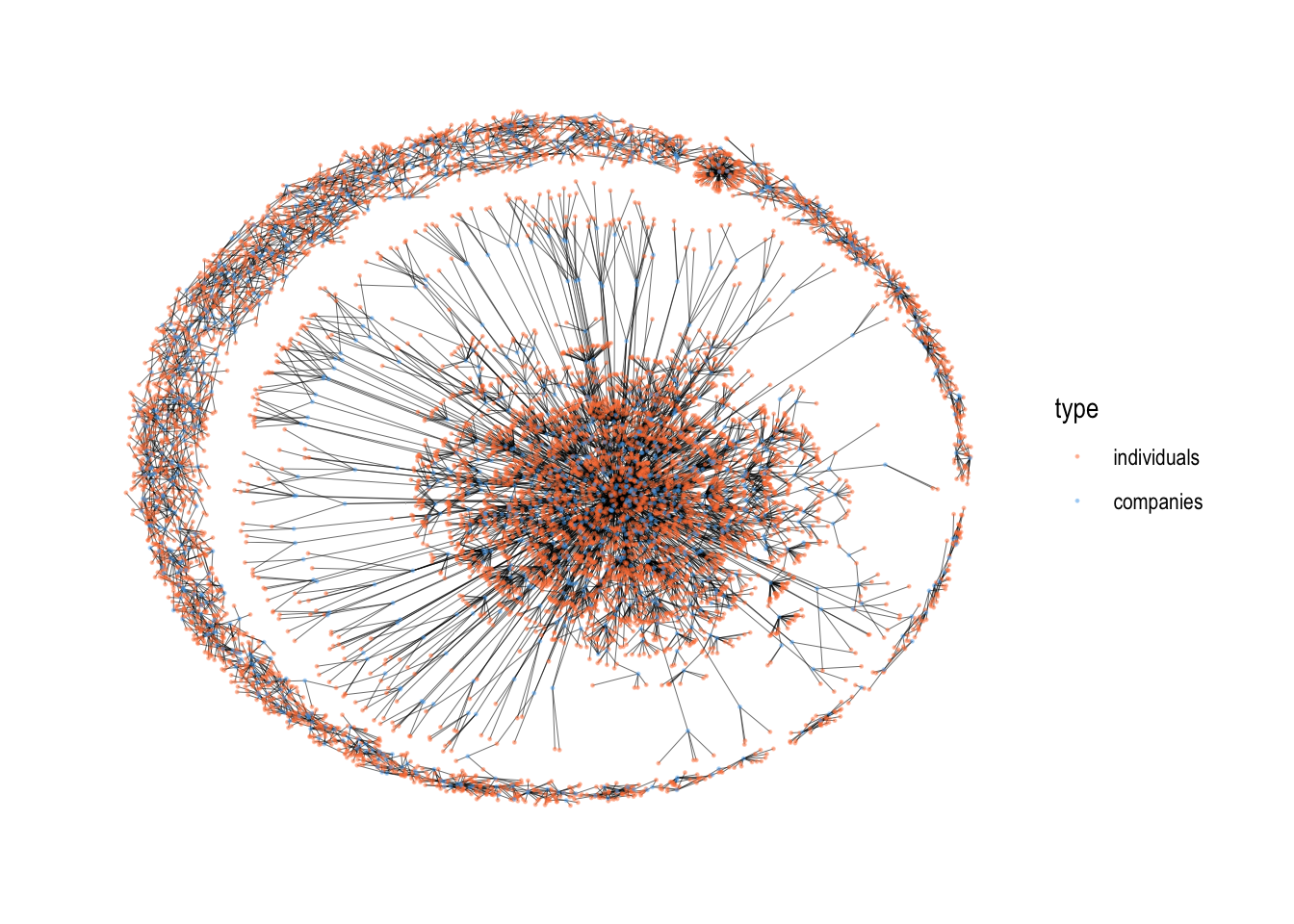
Despite the fact that we reduced the node size drastically, it is still difficult to view this network because of the limited page size. After all, it is a network with 8,090 nodes and 7,989 edges.

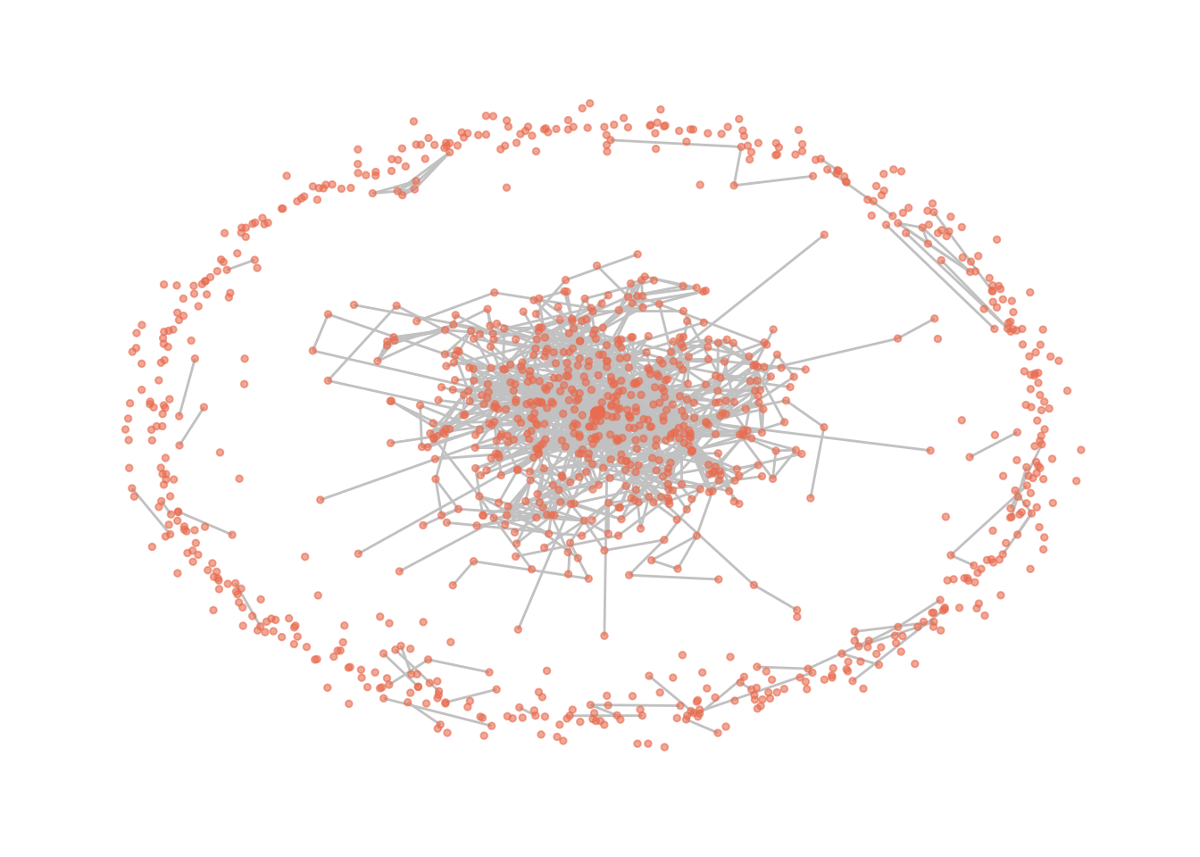
Let us also visualize the one-mode network of companies.

# Visualize the two mode graph
gr2 %>% 
#   # there are different layout types which changes the position of the nodes. For now, we only use this one called "kk" or "fr 
  ggraph(layout = "kk") +
  # draws edges
  geom_edge_link0(color = "gray80") +
  # draws nodes
  geom_node_point(size=1, alpha = 0.6, color = "salmon2") +
  theme_graph()

R-scripts #

To practice a little more, you can download an empty exercise sheet. You can also find a filled out cheat sheet below.